
Lab 2 Solutions
Gather round, for I shall tell a tale old as time. Long, long ago, astronomers gazed at the heavens, and with naught but their eyes, recorded the positions of the stars they saw there. Then, with the telescope, long, heavy contraptions which reached for the skies like an outstretched arm, (thanks, f/20 focal lengths) they gazed through eyepieces in freezing domes, falling, on occasion, to their deaths from cages suspended at prime foci.
Next came glass – emulsion plates – which upon extended exposure revealed upon their ghostly frames the splotches of stars and soon, galaxies and nebulae. Many a grad student, of course, spent their nights twiddling thumbs over micrometer dials to keep these stars in place. Manual guiding… this story teller shudders to imagine it. And yet, even then, with permanent record, no measure could be made that weren’t ‘tween the eyes of an observer, peering at the glass through magnifying eyepiece, assigning grades of brightness and, amazingly, pretty much nailing the spectral classification of stars by their absorption features.
And after this painstaking work, came the earliest CCDs, fractured by detector failures, riddled with readout noise, consumed by cosmic ray hits, laid low by low quantum efficiencies.
Now… we use Python.
Astronomical images are, in some sense, the bread and butter of astronomy. While we now obtain data in myriad ways, from gravitational waves to neutrinos, from spectra to polarimetry, the basic tenant of astronomy (and it's most recongizable public impact) is the images we make of the sky.
That is why the first science topic we’ll be tackling is imaging. And along the way, we’ll learn how astropy makes our lives so much easier when dealing with images, and how to use robust functions to perform the analyses one might want to carry out on images (after we’re done admiring their beauty).
Part I: If the glove FITS
Many of you are probably familiar with the FITS standard. It stands for Flexible Image Transport System, and for all intents and purposes, it acts as a container (much like a zip file). Within it, one can store several kinds of information: images (2d arrays of values), as the name implies, headers (dictionary like objects with metadata), and sometimes tabular data as well. A FITS file can contain any number of extensions, which just refer to “slots” where stuff is stored. Every “slot” has a header attribute and a data attribute. Thus, you could store a hundred astronomical images in 1 file, each with a different extension and a different header describing the image in that slot.
Tip
Contextual clues are important when dealing with FITS files. Files that are explicitly single images almost always have the image stored in the 0th extension, while files that are explicitly table data tend to have the table stored in the 1st extension (with the 0th empty).
The FITS standard is pretty old, and may be retired soon, but almost all ground based telescopes still use it for their native image output, so it behooves us to know how to get image data out of FITS files.
Problem 1: Loading a FITS file
Write a function which takes as its argument a string filepath to a FITS file, and should have an optional argument to set the extension (default 0). It should then load the given extension of that fits file using a context manager, and return a tuple containing the header and data of that extension.
The function should have documentation that describes the inputs and outputs. Documentation is incredibly important when writing code, both in-line and (# comments) and at the top of functions, methods, and classes.
In this class, we’ll be using Sphinx-compatible documentation written in the Numpy/Scipy style. There are several reasons to do this.
It is a user-friendly and write-friendly, readable documentation format that is easy to add to your functions.
It can be rendered by Sphinx, the most popular automatic documentation renderer. If you’ve ever read the online documentation pages for functions in, e.g., numpy and scipy, those pages were rendered automatically based on the docstrings of the functions in question. This is possible with tools like Sphinx, but the documentation must be formatted correctly for this to work.
In the cell below, I’ve provided a dummy function which takes in any number of inputs (mininum 3) and chooses a random input to return. The formatting of the documentation is shown there (as well as in the link above).
import numpy as np

def random_return(a,b,c,*args):
    '''
    A function which requires three inputs which are floats, accepts any number of additional inputs (of any kind), and returns one randomly chosen input.

    Parameters
    ----------
    a: int
        description of this integer input
    b: int
        description of this integer input
    c: int
        description of this integer input
    *args: tuple
        any additional arguments get stored here

    Returns
    -------
    choice
        The randomly selected input (type not specified)
    '''
    full_input_list = [a,b,c] + list(args)
    choice = np.random.choice(full_input_list)
    return choice
random_return(1,5,4,6,4,21,6)
5
When our function has been imported in some code, we can use the help command to see the documentation at any time:
help(random_return)
Help on function random_return in module __main__:

random_return(a, b, c, *args)
    A function which requires three inputs which are floats, accepts any number of additional inputs (of any kind), and returns one randomly chosen input.

    Parameters
    ----------
    a: int
        description of this integer input
    b: int
        description of this integer input
    c: int
        description of this integer input
    *args: tuple
        any additional arguments get stored here

    Returns
    -------
    choice
        The randomly selected input (type not specified)
You will also notice my use of *args in this function. This allows me to enter additional function arguments. Similar is **kwargs, which allows additional arguments tied to an input keyword. The former gets stored in a tuple, while the latter gets stored in a dictionary. We’ll be using these a lot in class — you can refresh or learn the basics in Section 2.8 of the chapter on functional programming here.
So as a brief overview of documentation, it contains
A brief summary of the function
The word Parameters with the next line having underlines of the same length
arguments, which are followed by a colon and the data type(s). On the next line, indented, descriptions of the arguments
The word Returns, with the same underline scheme
The returned objects, labeled the same way as the input.
Also above, we saw how to format when no data type is specified. There, additional inputs could’ve been any data type, so we can’t be sure what the output will be. The main thing we didn’t cover is optional arguments. Those are set like this:
a: int, optional
    Description of the thing. (default 5)
So we mark it as optional, and then give the default for it.
With that, you’re ready to write and document your code below. All functions you write in this class should have documentation.
# Solution
from astropy.io import fits
import os
def load_fits(fpath,extension=0):
    '''
    Function to load a FITS file into python

    Parameters
    ----------
    fpath: str
        path to the FITS file to load. must end in .fit/.fits/.FIT/.FITS
    extension: int (optional)
        extension of the FITS file to load. (default 0)

    Returns
    -------
    header: dict_like
        the read in header of the chosen extension, as a python dictionary
    data: array_like
        the data contained in the extension, whether an image or table.
    '''
    with fits.open(fpath) as hdu:
        header = hdu[extension].header
        data = hdu[extension].data
    return header, data
Problem 2: Data I/O
Problem 2.1
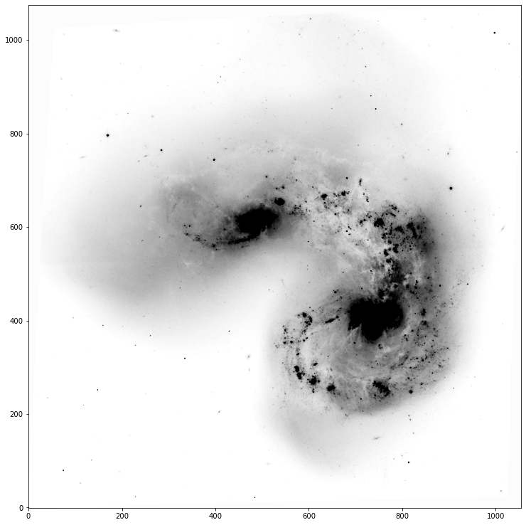
Using the function you created above, read in the header and data of the file antenna_Rband.fits which came with the lab assignment.
Note
While this may seem small, the fact that your read-in is now one line instead of ~5 does improve your efficiency! But only if you use your function enough times to overcome the initial time spent writing it…
We also have the flexibility to take our function and give it more features over time, which we will do in this class.
# Solution
head,data = load_fits('antenna_Rband.fits')
Problem 2.2
Next, we neex to plot the image data. There are several operations that we almost always perform when plotting astronomical data, as well as several user-preferences for how we “by default” plot images before we begin tweaking things. If you spend any time as an astronomer, you will plot quite literally thousands of images — why set all these settings every time, when we can write a handy function to do it for us?
Write a function which takes in as input arguments
an image (2D array or masked array)
as well as the following optional arguments (so set a default)
figsize (default (15,13) )
cmap (default ‘gray_r’)
scale (default 0.5)
**kwargs (see here)
Inside the function, create figure and axes objects using plt.subplots(). When working in notebooks, it is often useful to set the figsize argument of subplots to a nice large-ish value, such as (15,13), which will make the image fill most of the notebook. Since your function has set figsize as an argument, you can feed figsize directly into the subplots call, so that a user of the function can leave the default or set their own.
Next, use ax.imshow() to actually plot the image. You’ll want to save the output of this, e.g., im = ax.imshow(...). In this plotting call, set imshow’s argument origin='lower'. We always want to do this when dealing with imaging, as we want (0,0) to be a coordinate.
Note
By default, matplotlib uses a “matrix-style” plotting, where 0 of the y axis is in the top left corner, and 0 of the x axis is in the bottom left corner.
Also within the call to imshow(), feed in the cmap from your function (i.e., cmap=cmap). The other critical imshow() arguments are vmin and vmax, which sets the saturation points (and thus the contrast) of the image.
We haven’t set vmin and vmax as arguments of our outer function, but because of kwargs, we can still create a default here that can be overriden from outside.
As a default, within your function, calculate the mean and standard deviation of the image. Set some temporary variables with the quantities mu - scale*sigma and mu + scale*sigma (where here mu is the calculated mean and sigma is the calculated std dev, and scale was the optional input). Next, check the kwargs dictionary (which will exist in your function because we added the packing argument **kwargs to our function. IF vmin and vmax are in this dictionary, plug those into your imshow command. Otherwise, use the values determined by the calculation above. Bonus point for accomodating either no vmin/vmax entered, just vmin or vmax, or both (using the calculated values when things aren’t provided).
Your function should return the created fig and ax objects so the user can continue to tweak them.
Run your function and test its outputs. Once you’re satisfied it’s working, use it to plot the provided data. Find either a vmin/vmax pair, or a choice of scale which makes the image look pretty!
import matplotlib.pyplot as plt
import numpy as np

#Solution

def implot(image,figsize=(15,13),cmap='gray_r',scale=0.5,**kwargs):
    '''
    Plot an astronomical image, setting default options and easy tweaking of parameters

    Parameters
    ----------
    image: array_like
        2D array containing an astronomical image to be plotted. Cutouts should be input as cutout.data.
    figsize: tuple, optional
        figure size to use. Default: (15,13)
    cmap: str, optional
        Colormap to use for the image. Default: 'gray_r'
    scale: float, optional
        By default, function will scale image to some number of standard deviations about the mean pixel value. Scale sets this number (or fraction). Default: 0.5.
    **kwargs
        Additional arguments are passed to matplotlib plotting commands. Currently supported: vmin, vmax.

    Returns
    -------
    fig, ax
        figure and axes objects containing currently plotted data.
    '''
    fig, ax = plt.subplots(figsize=figsize)
    mu = np.mean(image)
    s = np.std(image)
    dvmin = mu - scale*s
    dvmax = mu + scale*s
    if all(['vmin','vmax']) in kwargs.keys():
        im = ax.imshow(image,origin='lower',cmap=cmap,vmin=kwargs['vmin'],vmax=kwargs['vmax'])
    elif 'vmin' in kwargs.keys():
        im = ax.imshow(image,origin='lower',cmap=cmap,vmin=kwargs['vmin'],vmax=dvmax)
    elif 'vmax' in kwargs.keys():
        im = ax.imshow(image,origin='lower',cmap=cmap,vmin=dvmin,vmax=kwargs['vmax'])
    else:
        im = ax.imshow(image,origin='lower',cmap=cmap,vmin=dvmin,vmax=dvmax)

    return fig, ax
fig, ax = implot(data,scale=2.5,vmin=10,vmax=100)
Problem 2.3
Copy your function down, we’re going to keep messing with it.
So far, we’ve made it so that with a simple function call and, potentially, with just the input of an image array, we get out a nice plot with a scaling, colormap, and origin selection. In this section, we are going to allow (optionally) for a colorbar to be added to the figure. We’re also going to add in the ability for the figure to be plotted in celestial coordinates (i.e., RA and DEC) instead of pixel units, if information about the image (via the world coordinate system, WCS) exists in the image header.
Note
Generally, WCS information is present in the headers of published images like the one here, but not present in raw data gathered at the telescope. This is because images need to undergo a process known as plate solving to determine both the direction (coordinates) toward the image, as well as the pixel scale (i.e., how many arcseconds per pixel in the image).
Add three new optional arguments to your function.
colorbar = False
header = None
wcs = None
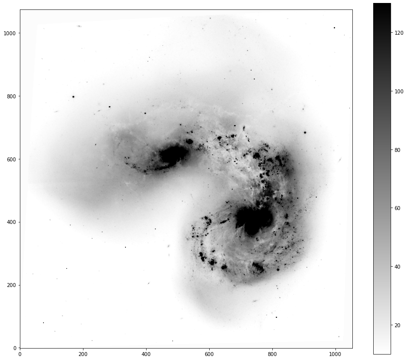
Let’s start with the colorbar. At the end of your plotting commands, check if colorbar=True, and if so, create a colorbar via plt.colorbar(), setting the mappable argument to whatever you saved the output of ax.imshow() into above. Also set the ax argument to be your ax; this will tell matplotlib to steal a bit of space from that axis to make room for the colorbar.
def implot(image,figsize=(15,13),cmap='gray_r',scale=0.5,colorbar=False,header=None,wcs=None,**kwargs):
    '''
    Plot an astronomical image, setting default options and easy tweaking of parameters

    Parameters
    ----------
    image: array_like
        2D array containing an astronomical image to be plotted. Cutouts should be input as cutout.data.
    figsize: tuple, optional
        figure size to use. Default: (15,13)
    cmap: str, optional
        Colormap to use for the image. Default: 'gray_r'
    scale: float, optional
        By default, function will scale image to some number of standard deviations about the mean pixel value. Scale sets this number (or fraction). Default: 0.5.
    colorbar: bool, optional
        Whether to add a colorbar or not. Default: False
    header: dict, optional
        If input, function will attempt to create a WCS object from header and plot in celestial coordinates. Default: None
    wcs: WCS object
        If input, the function will plot using a projection set by the WCS. Default: None
    **kwargs
        Additional arguments are passed to matplotlib plotting commands. Currently supported: vmin, vmax.

    Returns
    -------
    fig, ax
        figure and axes objects containing currently plotted data.
    '''
    fig, ax = plt.subplots(figsize=figsize)
    mu = np.mean(image)
    s = np.std(image)
    dvmin = mu - scale*s
    dvmax = mu + scale*s
    if all(['vmin','vmax']) in kwargs.keys():
        im = ax.imshow(image,origin='lower',cmap=cmap,vmin=kwargs['vmin'],vmax=kwargs['vmax'])
    elif 'vmin' in kwargs.keys():
        im = ax.imshow(image,origin='lower',cmap=cmap,vmin=kwargs['vmin'],vmax=dvmax)
    elif 'vmax' in kwargs.keys():
        im = ax.imshow(image,origin='lower',cmap=cmap,vmin=dvmin,vmax=kwargs['vmax'])
    else:
        im = ax.imshow(image,origin='lower',cmap=cmap,vmin=dvmin,vmax=dvmax)
    if colorbar:
        cbar = plt.colorbar(im,ax=ax)
    return fig, ax
fig, ax = implot(data,scale=2.5,vmin=10,vmax=100,colorbar=True)
Tip
You’ll notice in my solution, the colorbar is matching the figure height, rather than the axis height. If that bugs you like it bugs me, check out this solution from StackOverflow, which you can adapt within your function to make the cbar match the axis height.
In order to plot in RA and DEC coordinates, we need to first have an astropy WCS object associated with the image in question. You can import WCS from astropy.wcs. WCS objects are created from the headers of plate-solved fits files. In our function, we allow the user to input either a header or a WCS object directly.
Within your function, check if WCS is input – if it is, we’re good to go and can safely ignore header (even if it is provided). If instead only header is provided, use the WCS() function to create a new wcs object from that header.
Tip
You’ll want to do this at the very top of your function.
We now need to move our fig, ax = .... creation line into an if-statement. If we are using WCS “stuff”, you’ll need to set a projection for your plot that uses the wcs. This is accomplished as follows:
fig, ax = plt.subplots(...,subplot_kw={'projection':wcs})
where wcs is whatever you’ve named the output of WCS(header) or is the WCS input directly into the function.
from astropy.wcs import WCS

def implot(image,figsize=(15,13),cmap='gray_r',scale=0.5,colorbar=False,header=None,wcs=None,**kwargs):
    '''
    Plot an astronomical image, setting default options and easy tweaking of parameters

    Parameters
    ----------
    image: array_like
        2D array containing an astronomical image to be plotted. Cutouts should be input as cutout.data.
    figsize: tuple, optional
        figure size to use. Default: (15,13)
    cmap: str, optional
        Colormap to use for the image. Default: 'gray_r'
    scale: float, optional
        By default, function will scale image to some number of standard deviations about the mean pixel value. Scale sets this number (or fraction). Default: 0.5.
    colorbar: bool, optional
        Whether to add a colorbar or not. Default: False
    header: dict, optional
        If input, function will attempt to create a WCS object from header and plot in celestial coordinates. Default: None
    wcs: WCS object
        If input, the function will plot using a projection set by the WCS. Default: None
    **kwargs
        Additional arguments are passed to matplotlib plotting commands. Currently supported: vmin, vmax.

    Returns
    -------
    fig, ax
        figure and axes objects containing currently plotted data.
    '''
    if (header==None) and (wcs==None):
        fig, ax = plt.subplots(figsize=figsize)
    elif wcs is not None:
        fig, ax = plt.subplots(figsize=figsize,subplot_kw={'projection':wcs})
        ax.set_xlabel('Right Ascension [hms]',fontsize=15)
        ax.set_ylabel('Declination [degrees]',fontsize=15)
        ax.coords.grid(color='gray', alpha=0.5, linestyle='solid')
    elif header is not None:
        for i in header.keys():
            if i.startswith('A_'):
                del header[i]
            elif i.startswith('B_'):
                del header[i]
        header = strip_SIP(header)
        wcs = WCS(header)
        fig, ax = plt.subplots(figsize=figsize,subplot_kw={'projection':wcs})
        ax.set_xlabel('Right Ascension [hms]',fontsize=15)
        ax.set_ylabel('Declination [degrees]',fontsize=15)
        ax.coords.grid(color='gray', alpha=0.5, linestyle='solid')
    mu = np.mean(image)
    s = np.std(image)
    dvmin = mu - scale*s
    dvmax = mu + scale*s
    if all(['vmin','vmax']) in kwargs.keys():
        im = ax.imshow(image,origin='lower',cmap=cmap,vmin=kwargs['vmin'],vmax=kwargs['vmax'])
    elif 'vmin' in kwargs.keys():
        im = ax.imshow(image,origin='lower',cmap=cmap,vmin=kwargs['vmin'],vmax=dvmax)
    elif 'vmax' in kwargs.keys():
        im = ax.imshow(image,origin='lower',cmap=cmap,vmin=dvmin,vmax=kwargs['vmax'])
    else:
        im = ax.imshow(image,origin='lower',cmap=cmap,vmin=dvmin,vmax=dvmax)
    if colorbar:
        cbar = plt.colorbar(im,ax=ax)
    ax.tick_params(direction='in',length=9,width=1.5,labelsize=15)

    return fig, ax
Warning
In this case, we will get an error from our function that happens because of some distortion coefficient nonsense between astropy and drizzled HST images. Since it’s not pertinent to our lab, I’m providing below a snippet of code you should use to fix your header before running WCS(header).
def strip_SIP(header):
    A_prefixes = [i for i in header.keys() if i.startswith('A_')]
    B_prefixes = [i for i in header.keys() if i.startswith('B_')]
    for a,b in zip(A_prefixes,B_prefixes):
        del header[a]
        del header[b]
    return header
fig, ax = implot(data,scale=2.5,header=head,vmin=10)
WARNING: FITSFixedWarning: 'datfix' made the change 'Set MJD-OBS to 53207.000000 from DATE-OBS'. [astropy.wcs.wcs]
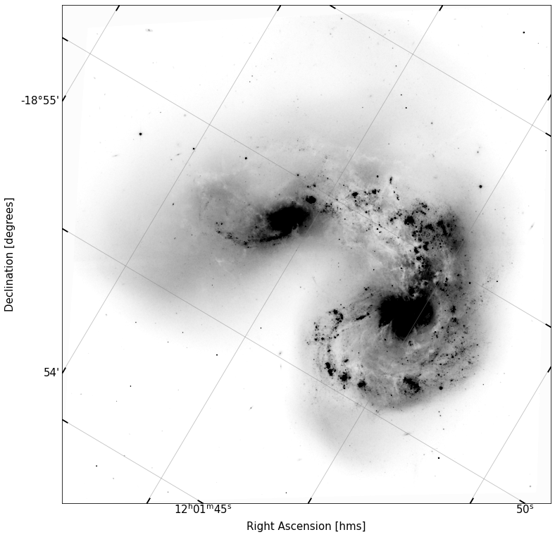
If this worked correctly, when you add the header you read in from our image, you should now see the axes of your plot change from pixels to pos.eq.ra and pos.eq.dec. We’re now looking at actual on-sky coordinates! Yay!
Within the if-blocks of your function that sets the ax to be a wcs projection, set the \(x\) and \(y\) labels to read “Right Ascension [hms]” and “Declination [degrees]” in fontsize 15.
Lastly, to polish things off, use ax.tick_params() to set inward, larger ticks, and increase the axis tick label size to 15.
Note
You’ll notice (especially with larger ticks) that the are not perpendicular to the axes spines. This is because this particular image has been rotated with respect to the standard celestial coordinate axes. This can be seen more clearly if you add the following to your function:
ax.coords.grid(color='gray', alpha=0.5, linestyle='solid'). Try doing that, adding an optional keyword to your function called ‘grid’ and enabling this command if it is set.
Tip
To check if a condition is true (e.g, if condition == True:), you can just type if condition:
It’s taken us some time, but this image could now be placed in a scientific publication. And, since we have a handy function for it, we can make images that look this nice on the fly with a short one line command, yet still have a lot of flexibility over many important inputs. And of course, the figure and axes objects are returned, so one could run this function and then continue tweaking the plot after the fact.
Note
As a final note, I want to draw your attention to the fact that once you use the wcs projection on some plot, it’s no longer a normal ax object, it’s a wcsax object. This makes changing certain elements of those axes a little more involved than for a standard one. I use this page and the others linked there when doing so.
Problem 3: Cutouts and Aperture Photometry
When working with astronomical images, like the one we’ve been using in this lab, it is often advantageous to be working with a cutout – a chunk of the image centered on a certain coordinate, and of a certain size. For example, if there is an HII region or star cluster of interest in the above image, we may like to zoom in on it to examine it more closely.
Now that we’ve switched over to using celestial coordinates instead of pixels as our projection frame, zooming in on a region is not as simple as slicing our array, e.g., image[500:700,200:550]. On the plus side, the framework we’ll learn here is very robust, and will allow for all sorts of useful measurements.
To make a cutout, we’ll need the Cutout2D module within astropy, which I’ll import below. To provide the position of the cutout, we need to be able to feed in astronomical coordinates. For this, we’ll use SkyCoord, a module in astropy.coordinates. Finally, we’ll need to integrate the units module in astropy to successfully create coordinate objects.
from astropy.nddata import Cutout2D
from astropy.coordinates import SkyCoord
import astropy.units as u
Let’s start with a SkyCoord object. There are several coordinate systems used in astronomy, e.g., Galactic coordinates (\(b\), \(l\)), Equatorial (\(RA\), \(DEC\)). The most common (especially in any extragalactic setting) is RA and DEC (as you can see in the image you’ve plotted already).
The documentation for SkyCoord is solid, and worth reading.
The general way we create these objects is, e.g.,
coord = SkyCoord('12:01:53.6 -18:53:11',unit=(u.hourangle,u.deg))
Tip
You can input various types of strings and formattings for the coordinates, just be sure to specify the units as shown above. The documentation shows the various methods.
Problem 3.1
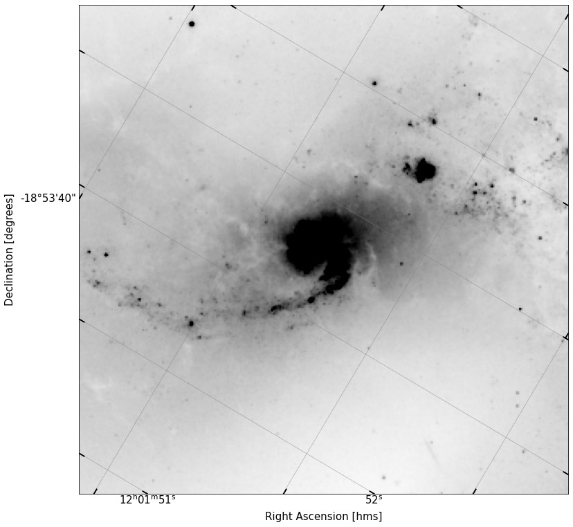
In this case, the coordinates I set above are for NGC 4039, which is the smaller of the two galaxies in the image we’re using.
Note
If at any point you’re trying to make a coordinate object for a well known galaxy/object, try, e.g., coord = SkyCoord.from_name('NGC 4038'), and ususally that will work!
In the cell below, use the coordinate we’ve created, plus a size (use 1x1 arcminutes), and the wcs object for our image, to create a Cutout2D object.
#cutout = # your code here
# Solution

cutout = Cutout2D(data,coord,size=(1*u.arcmin,1*u.arcmin),wcs=WCS(head))
WARNING: FITSFixedWarning: 'datfix' made the change 'Set MJD-OBS to 53207.000000 from DATE-OBS'. [astropy.wcs.wcs]
Now, use your fancy new function to plot the new cutout.
Note
Cutout objects contain the image and their own wcs, accessible via, e.g., cutout.data and cutout.wcs.
implot(cutout.data,scale=2,vmin=10,wcs=cutout.wcs)
(<Figure size 1080x936 with 1 Axes>,
 <WCSAxesSubplot:xlabel='Right Ascension [hms]', ylabel='Declination [degrees]'>)
Problem 3.2
We’re now going to do some aperture photometry.
Definition
Aperture Photometry is the process of defining a region on an image (generally, but not always circular), and measuring the sum pixel value within that region. The region is known as an aperture, and the “collapsing” of the 2D spatial information about counts in each pixel into a single number is known as photometry.
Below, I provide a new coordinate, this time centered on the region between the two galaxies. Make a new cutout of that region (again, 1x1 arcmin), and plot it.
new_coord = SkyCoord('12:01:55.0 -18:52:45',unit=(u.hourangle,u.deg))
#Solution
new_cutout = Cutout2D(data,new_coord,size=(1*u.arcmin,1*u.arcmin),wcs=WCS(head))
WARNING: FITSFixedWarning: 'datfix' made the change 'Set MJD-OBS to 53207.000000 from DATE-OBS'. [astropy.wcs.wcs]
implot(new_cutout.data,scale=2,vmin=10,wcs=new_cutout.wcs)
(<Figure size 1080x936 with 1 Axes>,
 <WCSAxesSubplot:xlabel='Right Ascension [hms]', ylabel='Declination [degrees]'>)
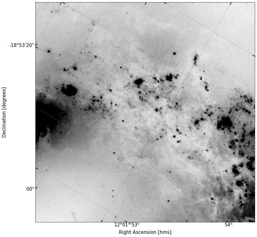
In this region, there are a lot of blobby looking roughly circular sources — Some of the larger ones are HII star forming regions, the smaller ones are likely stars.
Often, for calibration purposes, we’d need to create apertures around all those sources in the image. We definitely don’t want to do that by hand! Instead, we’re going to use the sep package.
Note
Simply pip install sep inside your a330 environment terminal to get it installed, you should then be able to import it.
import sep
There are three steps to performing aperture photometry with sep, which are detailed in it’s documentation.
Estimate the background
Find Sources
Perform Aperture Photometry
Using the instructions presented in the documentation linked, measure the background of the cutout image, and run the source extractor on it. Don’t forget to subtract the background before running the extractor!
To do this, write a function that takes as input the data (in this case, a cutout.data object and a threshold scale (to be multiplied by the globalrms, and performs these steps, returning the objects array. Don’t forget to document it!
Hint
I used a threshold value of 2.0, and got ~100 objects.
Warning
When I ran this, I got an error that my “array was not C-contiguous.” I found the solution to this issue in this stackoverflow post. Loosely, sep uses C-bindings to actually run the heavy lifting code in C rather than Python (it’s faster). This means input arrays must be arranged in physical memory the way C is used to. This particular array was not, but it is easy to order it this way.
# Solution

def run_sep(data,thresh_scale=2.0):
    '''
    Sep wrapper... runs a basic set of sep commands on a given image

    Parameters
    ----------
    data: array_like
        the input image
    thresh_scale: float
        a scaling parameter used by sep to determine when to call something a source (see sep documentation)

    Returns
    -------
    objects: numpy struct array
        numpy structured array containing the sep-extracted object locations, etc.
    '''
    data_corder = data.copy(order='C')
    bkg = sep.Background(data_corder)
    back = bkg.back()
    data_bg_sub = data - back
    c_copy = data_bg_sub.copy(order="C")

    thresh = thresh_scale * bkg.globalrms
    objects = sep.extract(c_copy, thresh)
    return objects
Run your function and store the output in a variable called objects. You should now have an object array containing many detected sources.
objects = run_sep(new_cutout.data)
len(objects)
<ipython-input-31-36a3a31cfa1e>:26: DeprecationWarning: `np.int` is a deprecated alias for the builtin `int`. To silence this warning, use `int` by itself. Doing this will not modify any behavior and is safe. When replacing `np.int`, you may wish to use e.g. `np.int64` or `np.int32` to specify the precision. If you wish to review your current use, check the release note link for additional information.
Deprecated in NumPy 1.20; for more details and guidance: https://numpy.org/devdocs/release/1.20.0-notes.html#deprecations
  objects = sep.extract(c_copy, thresh)
103
The positions of the determined sources are stored in the output structured array and can be indexed with, e.g., objects['x'] and objects['y']. Replot your image of the cutout, but now circle the positions of all your detected sources. Do they line up with actual point sources in the image?
Hint
Try using ax.plot, setting your symbol to ‘o’, your color to ‘None’, your marker edge color (mec) to some color, and the marker size (ms) to some largeish value, for a quick way to circle objects.
fig, ax = implot(new_cutout.data,scale=2,vmin=10,wcs=new_cutout.wcs)
ax.plot(objects['x'],objects['y'],'o',ms=15,color='None',mec='r')
[<matplotlib.lines.Line2D at 0x7fb00834b160>]
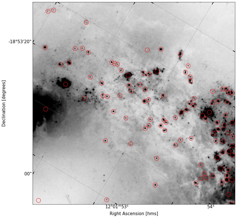
It looks like we’ve done a pretty adequate job finding the sources in this field – there’a a few that got missed, and a few we might want to remove, but overall, this is pretty solid.
We need to start working with these objects we’ve found. While sep can perform aperture photometry itself (reading the docs, you can see it is simple to feed in the objects and a pixel radius), we’re going to be a bit more careful about things. To better visualize and work with this data, I’d like it to be a pandas DataFrame. We’re going to be using those a lot in this course. Converting a numpy structured array to a dataframe is simple: I provide the code below. Run it, and then simply type df in a new cell to see a nicely formatted pandas table of our objects.
import pandas as pd
df = pd.DataFrame(objects)
df
| thresh | npix | tnpix | xmin | xmax | ymin | ymax | x | y | x2 | ... | cxy | cflux | flux | cpeak | peak | xcpeak | ycpeak | xpeak | ypeak | flag | |
|---|---|---|---|---|---|---|---|---|---|---|---|---|---|---|---|---|---|---|---|---|---|
| 0 | 13.807426 | 19 | 15 | 291 | 298 | 0 | 2 | 294.331652 | 0.748626 | 3.010990 | ... | 0.528804 | 612.740173 | 767.704102 | 55.058762 | 99.534592 | 294 | 0 | 294 | 0 | 2 |
| 1 | 13.807426 | 7 | 4 | 108 | 110 | 5 | 7 | 109.067891 | 6.332346 | 0.508919 | ... | -0.177127 | 143.963638 | 178.128448 | 28.999582 | 66.128693 | 109 | 6 | 109 | 6 | 0 |
| 2 | 13.807426 | 222 | 214 | 0 | 22 | 0 | 16 | 8.012520 | 5.514646 | 32.370749 | ... | 0.033329 | 3656.097412 | 3757.238525 | 21.895723 | 24.796696 | 1 | 1 | 1 | 6 | 2 |
| 3 | 13.807426 | 10 | 4 | 180 | 183 | 27 | 29 | 181.260591 | 28.091515 | 0.624076 | ... | 0.004285 | 455.730774 | 508.251770 | 93.388168 | 261.102325 | 181 | 28 | 181 | 28 | 0 |
| 4 | 13.807426 | 12 | 9 | 240 | 243 | 30 | 33 | 241.296235 | 31.149263 | 0.837190 | ... | 0.627759 | 476.430389 | 603.428528 | 72.289940 | 157.386230 | 241 | 31 | 242 | 31 | 0 |
| ... | ... | ... | ... | ... | ... | ... | ... | ... | ... | ... | ... | ... | ... | ... | ... | ... | ... | ... | ... | ... | ... |
| 98 | 13.807426 | 54 | 51 | 185 | 193 | 226 | 233 | 189.610462 | 229.462692 | 1.588913 | ... | 0.061697 | 4849.710938 | 4877.654785 | 626.254272 | 1383.217651 | 190 | 229 | 190 | 229 | 1 |
| 99 | 13.807426 | 670 | 592 | 152 | 187 | 212 | 250 | 169.199212 | 228.711439 | 62.010877 | ... | 0.003127 | 10656.494141 | 10797.801758 | 21.452864 | 27.849247 | 171 | 228 | 171 | 228 | 1 |
| 100 | 13.807426 | 13 | 10 | 77 | 81 | 268 | 271 | 78.812474 | 269.285180 | 1.357104 | ... | 0.780199 | 233.011490 | 273.878479 | 23.973366 | 43.442318 | 80 | 269 | 80 | 268 | 1 |
| 101 | 13.807426 | 8 | 6 | 21 | 23 | 285 | 287 | 21.845574 | 286.156461 | 0.543330 | ... | -0.990262 | 153.411697 | 204.978119 | 25.171600 | 50.913998 | 22 | 286 | 22 | 287 | 0 |
| 102 | 13.807426 | 7 | 4 | 29 | 31 | 287 | 289 | 30.329319 | 287.833190 | 0.443130 | ... | -1.248477 | 125.931458 | 152.977509 | 23.354290 | 42.604931 | 31 | 288 | 31 | 288 | 0 |
103 rows × 30 columns
With sep providing the first pass, we can cull a few objets from our sample that very clearly are not star forming regions. Using your DataFrame, plot the flux of each detected object using the flux column. You should have at least a few that are huge outliers, with dramatically more flux the rest.
plt.plot(df.flux,'.')
[<matplotlib.lines.Line2D at 0x7fafe87023a0>]
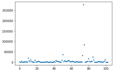
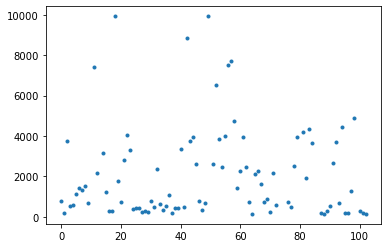
Write a function called remove_outliers that reads in a dataframe and a flux-min and flux-max. It should filter the dataframe to only include fluxes between the input values, and return the new dataframe. Then use this function on your data, choosing an appropriate cutoff.
# Solution

def remove_outliers(df,flux_min,flux_max):
    return df.loc[(df['flux']>flux_min)&(df['flux']<flux_max)]
df2 = remove_outliers(df,0,10000)
plt.plot(df2.flux,'.')
[<matplotlib.lines.Line2D at 0x7fb02abd3af0>]
df2
| thresh | npix | tnpix | xmin | xmax | ymin | ymax | x | y | x2 | ... | cxy | cflux | flux | cpeak | peak | xcpeak | ycpeak | xpeak | ypeak | flag | |
|---|---|---|---|---|---|---|---|---|---|---|---|---|---|---|---|---|---|---|---|---|---|
| 0 | 13.807426 | 19 | 15 | 291 | 298 | 0 | 2 | 294.331652 | 0.748626 | 3.010990 | ... | 0.528804 | 612.740173 | 767.704102 | 55.058762 | 99.534592 | 294 | 0 | 294 | 0 | 2 |
| 1 | 13.807426 | 7 | 4 | 108 | 110 | 5 | 7 | 109.067891 | 6.332346 | 0.508919 | ... | -0.177127 | 143.963638 | 178.128448 | 28.999582 | 66.128693 | 109 | 6 | 109 | 6 | 0 |
| 2 | 13.807426 | 222 | 214 | 0 | 22 | 0 | 16 | 8.012520 | 5.514646 | 32.370749 | ... | 0.033329 | 3656.097412 | 3757.238525 | 21.895723 | 24.796696 | 1 | 1 | 1 | 6 | 2 |
| 3 | 13.807426 | 10 | 4 | 180 | 183 | 27 | 29 | 181.260591 | 28.091515 | 0.624076 | ... | 0.004285 | 455.730774 | 508.251770 | 93.388168 | 261.102325 | 181 | 28 | 181 | 28 | 0 |
| 4 | 13.807426 | 12 | 9 | 240 | 243 | 30 | 33 | 241.296235 | 31.149263 | 0.837190 | ... | 0.627759 | 476.430389 | 603.428528 | 72.289940 | 157.386230 | 241 | 31 | 242 | 31 | 0 |
| ... | ... | ... | ... | ... | ... | ... | ... | ... | ... | ... | ... | ... | ... | ... | ... | ... | ... | ... | ... | ... | ... |
| 97 | 13.807426 | 20 | 16 | 16 | 20 | 230 | 234 | 17.861561 | 232.250039 | 0.998464 | ... | 0.087940 | 1223.592896 | 1285.245728 | 181.206024 | 462.152161 | 18 | 232 | 18 | 232 | 0 |
| 98 | 13.807426 | 54 | 51 | 185 | 193 | 226 | 233 | 189.610462 | 229.462692 | 1.588913 | ... | 0.061697 | 4849.710938 | 4877.654785 | 626.254272 | 1383.217651 | 190 | 229 | 190 | 229 | 1 |
| 100 | 13.807426 | 13 | 10 | 77 | 81 | 268 | 271 | 78.812474 | 269.285180 | 1.357104 | ... | 0.780199 | 233.011490 | 273.878479 | 23.973366 | 43.442318 | 80 | 269 | 80 | 268 | 1 |
| 101 | 13.807426 | 8 | 6 | 21 | 23 | 285 | 287 | 21.845574 | 286.156461 | 0.543330 | ... | -0.990262 | 153.411697 | 204.978119 | 25.171600 | 50.913998 | 22 | 286 | 22 | 287 | 0 |
| 102 | 13.807426 | 7 | 4 | 29 | 31 | 287 | 289 | 30.329319 | 287.833190 | 0.443130 | ... | -1.248477 | 125.931458 | 152.977509 | 23.354290 | 42.604931 | 31 | 288 | 31 | 288 | 0 |
93 rows × 30 columns
Re-plot the set of sources you have now, over the data.
fig, ax = implot(new_cutout.data,scale=2,vmin=10,wcs=new_cutout.wcs)
ax.plot(df2['x'],df2['y'],'o',ms=15,color='None',mec='r')
[<matplotlib.lines.Line2D at 0x7faff01129a0>]
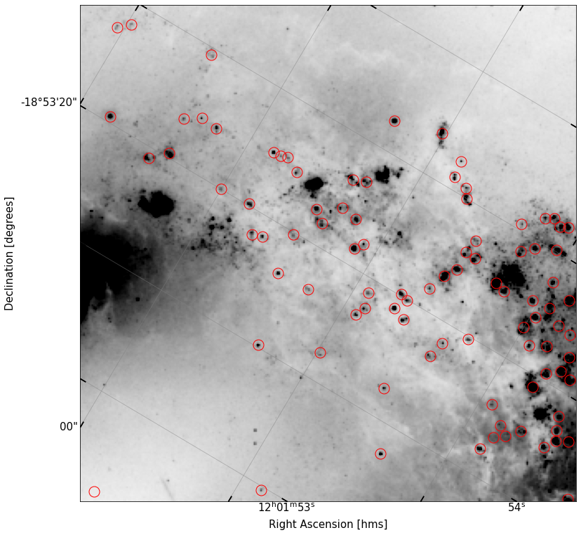
You should see that some of the circles which were over bright parts of the galaxy are no longer here.
Note
You may find that there are some visible sources which, despite tinkering, don’t get caught by sep. That’s okay – if we really wanted them, we could just go in and put down apertures by hand. Generally when performing a step like this in the field, we have a pre-determined set of points to use, because we have measured fluxes for them, and wish to flux calibrate our data.
Problem 4: Continuum Subtraction
At this point, we have the tools necessary to make flux measurements in apertures (at least, via sep – we will also learn how to do this with the photutils package). However, \(R\) band photometry of HII regions is not exceedingly interesting. More interesting is the flux in \(H\alpha\), an emission line caused by Hydrogen recombination. This line (at 6563 Angstrom) is located within the \(R\) band, and is imaged using a narrow filter compared ot \(R\).
The flux measured by an \(H\alpha\) filter contains both the flux from the emission line as well as the underlying continuum — essentially, the starlight from the galaxy. If we can get a clean measure of the flux in \(H\alpha\) (sans this continuum), we can make a direct estimate of the star formation rate of the system.
Problem 4.1
To do this, we need to access an \(H\alpha\) image, and then subtract off the continuum present (which we’ll infer from our \(R\) band image). Located in the lab directory is a file called antenna_Haband.fits. Use your fits loader function from above to read in this new image, create an equivalent sized and centered cutout to the \(R\) band data, and plot it, with the same sources found in the \(R\) band circled.
# Solution

head2, data2 = load_fits('antenna_Haband.fits')
head2 = strip_SIP(head2)
cutout_ha = Cutout2D(data2,new_coord,size=(1*u.arcmin,1*u.arcmin),wcs=WCS(head2))
WARNING: FITSFixedWarning: 'datfix' made the change 'Set MJD-OBS to 53207.000000 from DATE-OBS'. [astropy.wcs.wcs]
fig, ax = implot(cutout_ha.data,scale=0.7,vmin=1,wcs=cutout_ha.wcs)
ax.plot(df2['x'],df2['y'],'o',ms=15,color='None',mec='r')
[<matplotlib.lines.Line2D at 0x7fb02011d040>]
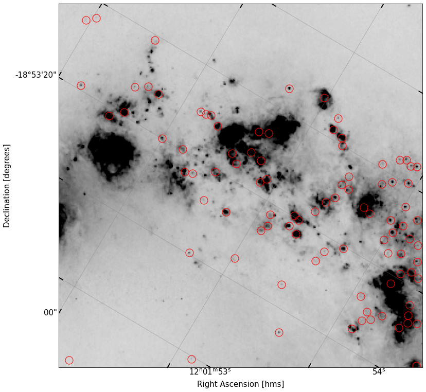
There’s a few interesting things to note right away here. Looking just north of the center of the image, there’s now a large amount of flux in \(H\alpha\) coming from some blobs which do not appear in the \(R\) band. This is likely due to the fact that by zero-ing in on the ionized gas, we can see the large envelopes of gas being lit up by the star formation in this region.
Note
The active merger scenario between these two galaxies is triggering a lot of star formation.
Problem 4.2
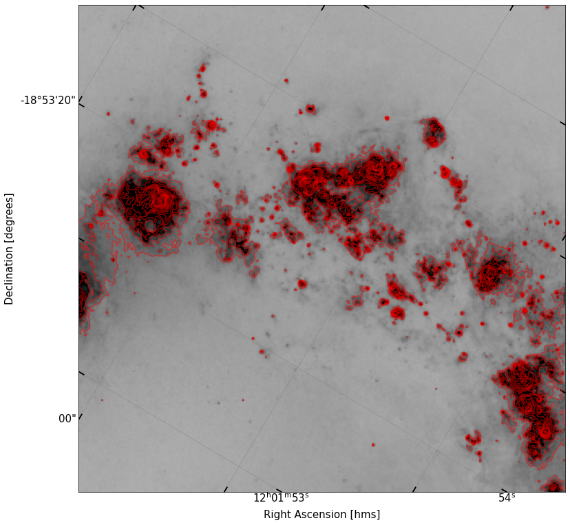
To get a better idea of how the \(H\alpha\) flux compares to the \(R\) band distribution, use the plt.contour() tool to measure contours of \(H\alpha\), drawing them over the
\(H\alpha\) image and tweaking the levels until you think you are well tracing the distribution. Then, plot those contours over the \(R\) band data instead.
Hint
It is often beneficial to use np.logspace() when defining contour levels, as it allows you to cover large dynamic range with fewer contours. You may also find it helpful to set your contour alpha to something < 1, to better see both the image underneath and the contours.
# Solution

fig, ax = implot(cutout_ha.data,scale=0.7,wcs=cutout_ha.wcs)
contours = ax.contour(cutout_ha.data,levels=np.logspace(1.8,4,20),colors='r',alpha=0.5)
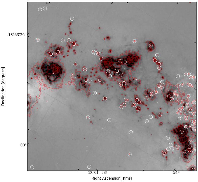
To help guide you, I’ve shown what I got for my plot below — you need not emulate it exactly. The blue box shown in the image will be useful to you in the next part of the problem.
fig, ax = implot(new_cutout.data,scale=2,vmin=10,wcs=new_cutout.wcs)
ax.contour(cutout_ha.data,levels=np.logspace(1.8,4,10),colors='r',alpha=0.5,transform=ax.get_transform(cutout_ha.wcs))
patch_cent = SkyCoord('12:01:53.7 -18:52:52',unit=(u.hourangle,u.deg))
patch = SkyRectangularAperture(patch_cent,0.27*u.arcmin,0.2*u.arcmin)
patch.to_pixel(wcs=new_cutout.wcs).plot(lw=3,color='C0');
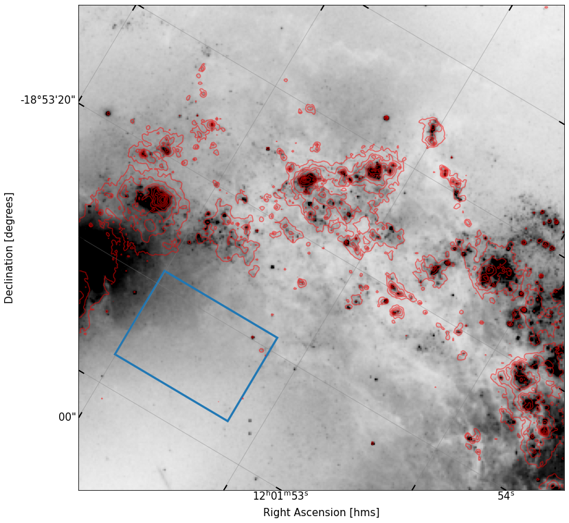
We can now see things a lot more clearly! It is obvious that the \(H\alpha\) contours trace the sources we were seeing in the \(R\) band, but that the gas is more extended around these clusters of sources, as we might expect.
Problem 4.3
We must now attempt a continuum subtraction of the data. We can’t simply subtract the \(R\) band from the \(H\alpha\) band, because the \(R\) band filter is much wider, and thus for similar exposure times, collects many more photons than the narrower \(H\alpha\) filter. Ideally, one could use a set of foreground stars (which are pure continuum sources in both images) to measure fluxes in both, and find a scaling constant. Here, all of the sources we see in this image are most likely actually HII regions. This means if we use them to scale between our images, we will likely oversubtract true flux.
Instead, what I’m going to do here (which may be slightly sketchy), is pick a “blank” region of continuum emission from the \(R\) band which has no \(H\alpha\) contours, and assert that this patch must have the same flux in both images. In the picture above, I indicated a blue rectangular patch on the sky. This is what we’ll be using to measure our continuum-to-narrowband ratio.
To make this patch, we’re going to use SkyRectangularAperture, from photutils. You can pip install photutils in your a330 environment if you don’t have it. Then do the following imports:
from photutils.aperture import SkyRectangularAperture
from photutils.aperture import aperture_photometry
As shown in it’s documentation, we need to feed in a SkyCoord position, as well as a width and a height.
I’ve provided the new coordinate to use below. Create a rectangle of your own, measuring \(0.27''\) by \(0.2''\). You can now use the aperture_photometry() function to measure the flux in your aperture, applied to a certain image. Using the documentation as needed, find the flux in this box for both the \(R\) band and \(H\alpha\) band data, and then determine the ratio between those values. Don’t forget about the wcs!
# Solution
patch_cent = SkyCoord('12:01:53.7 -18:52:52',unit=(u.hourangle,u.deg))
patch = SkyRectangularAperture(patch_cent,0.27*u.arcmin,0.2*u.arcmin)
patch_R_flux_table = aperture_photometry(new_cutout.data,patch,wcs=new_cutout.wcs)
patch_Ha_flux_table = aperture_photometry(cutout_ha.data,patch,wcs=cutout_ha.wcs)

R_flux = patch_R_flux_table['aperture_sum'][0]
Ha_flux = patch_Ha_flux_table['aperture_sum'][0]
fluxratio = R_flux/Ha_flux
print(fluxratio)
1.5917633100928574
According to my calculation, the \(R\) band sky is about 1.6 times brighter in our patch than the \(H\alpha\). So we can now use this ratio to perform our subtraction.
Note
This result is a bit strange to me. The R band filter is quite a bit larger, so I would expect the ratio to be larger. But the images may have different exposure times or reductions, which may be why this has happened.
Problem 4.4
Now, fill in the function below, which should read in your rectangular patch, the \(R\) band cutout object, and the \(H\alpha\) cutout object. Within the function, copy in the code that determines the ratio, and then use the ratio you found to scale your \(R\) band image, then subtract it from the \(H\alpha\) image. The function should return this new image array.
Plot up your continuum subtracted image using your implot() function, adding back in the apertures we found earlier and the contours we made from the full \(H\alpha\) image.
# Solution

def continuum_subtract(patch,Rcutout,Hacutout):
    '''
    Determines a continuum subtraction ratio between R band and Ha band image, then performs continuum subtraction

    Parameters
    ----------
    patch: SkyRectangularAperture object
        A rectangular patch defined in sky coordinates
    Rcutout: Cutout2D object
        Cutout2D object of the R band image
    Hacutout: Cutout2D object
        Cutout2D object of the Ha band image

    Returns
    -------
    sub_img: array_like
        continuum subtracted image
    '''
    patch_R_flux_table = aperture_photometry(Rcutout.data,patch,wcs=Rcutout.wcs) # flux table in rect R
    patch_Ha_flux_table = aperture_photometry(Hacutout.data,patch,wcs=Hacutout.wcs) # flux table in rect Ha
    R_flux = patch_R_flux_table['aperture_sum'][0] #extract flux
    Ha_flux = patch_Ha_flux_table['aperture_sum'][0] #extract flux
    fluxratio = R_flux/Ha_flux #determine ratio
    sub_img = Hacutout.data - (Rcutout.data/fluxratio) #perform subtraction
    return sub_img

sub_data = continuum_subtract(patch,new_cutout,cutout_ha)

fig, ax = implot(sub_data,scale=0.9,wcs=new_cutout.wcs)
ax.contour(cutout_ha.data,levels=np.logspace(1.8,4,10),colors='r',alpha=0.5,transform=ax.get_transform(cutout_ha.wcs))

ax.plot(df2['x'],df2['y'],'o',ms=15,color='None',mec='w')
[<matplotlib.lines.Line2D at 0x7fb008a479a0>]
What do you notice about the distribution of apertures with respect to the distribution of \(H\alpha\) gas? Is there a strong alignment of the \(R\) band sources and the gas? What does this imply about most of the \(R\) band sources?
Problem 4.5
Lastly, let’s load up the \(B\) band image. As you probably know, the \(B\) band traces bluer light, and thus will more preferentially see young, hot stars (whereas the \(R\) band traces the main sequence and turn off stellar distribution).
Load up the antenna_Bband.fits image, make a cutout, and plot it below. Make a new set of countours from your continuum subtracted \(H\alpha\) data, and overplot that onto the \(B\) band data. What do you see?
head3, data3 = load_fits('antenna_Bband.fits')
head3 = strip_SIP(head3)
cutout_B = Cutout2D(data3,new_coord,size=(1*u.arcmin,1*u.arcmin),wcs=WCS(head3))
WARNING: FITSFixedWarning: 'datfix' made the change 'Set MJD-OBS to 53207.000000 from DATE-OBS'. [astropy.wcs.wcs]
fig, ax = implot(cutout_B.data,scale=1.5,vmin=10,wcs=cutout_B.wcs)
ax.contour(sub_data,levels=np.logspace(1.3,4,10),colors='r',alpha=0.5,transform=ax.get_transform(cutout_ha.wcs))
<matplotlib.contour.QuadContourSet at 0x7f8236659b80>
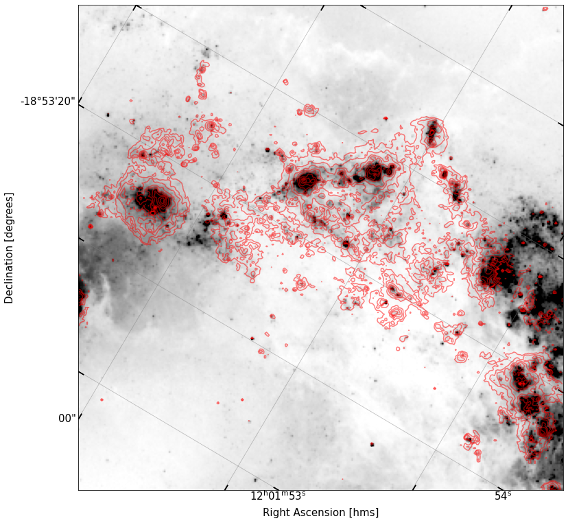
In my own image, there are some clusters of \(B\)-band flux that align well with the \(H\alpha\) contours, and some \(B\) band sources out on their own. It is unsurprising that there is a correspondance between them; excess in \(B\) light implies the prescence of UV radiation as well, from young O/B stars. It is this radiation responsible for ionizing the gas that is shining in \(H\alpha\), so the \(H\alpha\)-emitting gas should be loosely clustered around sources bright in the \(B\) band (the experiment would be even cleaner if we used, say, GALEX FUV data).
Bonus Question (up to 3 points)
If you want to take your analysis farther, try measuring some fluxes off of your continuum subtracted \(H\alpha\) data, placing several manual apertures down over the regions of highest \(H\alpha\) concentration (which also align with \(B\) band concentrations).
The measures you get from this will be in counts on the detector. We need to convert these counts into flux units (e.g., erg s\(^{-1}\) cm\(^{-2}\)). To do this,
pull the ‘PHOTFLAM’ keyword from the header of your \(H\alpha\) data
also pull the ‘EXPTIME’ value from the header.
Start by taking your fluxes in counts, multiplying by the PHOTFLAM value, and dividing by the EXPTIME value. This puts you in erg s\(^{-1}\) cm\(^{-2}\) per Angstrom. Thus, what we have is technically a flux density. To convert to a true flux, we’ll simply integrate over the bandpass… but for this example, let’s assume a constant flux across the bandpass, which for the ACS 658N filter (\(H\alpha\)), is 136.27 angstroms.
Once you have fluxes, use the distance to NGC 4038/9 to determine the luminosity in erg/s of your collective set of sources, and then use the \(SFR(H\alpha)\) calibration of Kennicut & Bell to convert to an SFR. How does your answer compare to, e.g.,
The SFR of the Milky Way?
The SFR of the Orion Nebula?
The SFR of the Tarantula Nebula?