Lab 6: Solutions¶

In this lab, we’ll work through some of the basics of using Pandas, using a few different tabular data sets. Ultimately, one need not do anything particularly fancy with DataFrames for them to be useful as data containers. But we would like to highlight a few extra abilities these objects have, that illustrate situations where we may actually have a strong reason to use pandas over another library.

Problem 1: HII regions + Planetary Nebulae measurements in M81¶

For our first data set, we’re going to look at a file (table2.dat), which contains measurements of the flux and intensity of various ions’ line emission from a set of known emitting objects (PNs and HII regions) in the M81 galaxy.

The columns of this file are name, ion, wl, flux, and I (intensity). Two of the columns are string-valued (name and ion), three are numerical-values (wl, flux, I). This mix of strings and floats tells us before we even decide how to read in this file that numpy data structures won’t be usable, as they demand all values in an array to have the same dtype.

Problem 1.1¶

Using the pd.read_csv() function shown in the lecture, read this data file into a dataframe called df, and print it.

Hint

You can get a “pretty” visualization of a dataframe by simply typing its name into a jupyter cell – as long as it’s the last line of the cell, the dataframe will print more nicely than typing print(df). This does not work outside of notebooks.

import numpy as np
import matplotlib.pyplot as plt
import pandas as pd
%matplotlib inline 
df = pd.read_csv('table2.dat')

df

	name	ion	wl	flux	rms	I
0	PN3m	[OII]	3727	373.9	58.6	517.3
1	PN3m	HeI	3805	0.0	0.0	0.0
2	PN3m	HI	3835	0.0	0.0	0.0
3	PN3m	[NeIII]	3869	0.0	0.0	0.0
4	PN3m	HeI	3889	0.0	0.0	0.0
...	...	...	...	...	...	...
1629	HII403	[ArIII]	7135	15.5	3.1	8.2
1630	HII403	[OII]	7320	0.0	0.0	0.0
1631	HII403	[OII]	7330	0.0	0.0	0.0
1632	HII403	[ArIII]	7751	0.0	0.0	0.0
1633	HII403	[SIII]	9069	51.1	3.7	17.3

1634 rows × 6 columns

Problem 1.2¶

Though it doesn’t show up in the clean representation above, the strings associated with the name and ion columns above have trailing and leading spaces that we don’t want.

Use a list comprehension to modify the data frame such that each value in the name and ion columns are replaced with a .strip() version of themselves.

df['name'] = [i.strip() for i in df.name]
df['ion'] = [i.strip() for i in df.ion]

Problem 1.3¶

Write a function select_object which takes in as an argument the name of an HII region or planetrary nebula, and filters the dataframe for only the entries for that object using df.loc[]. Consider having the dataframe be an optional argument you set to df, the dataframe we are working with.

Have your function take in an optional argument drop_empty=True which additionally selects only those rows where the flux/intensity is not zero.

def select_object(name,df=df,drop_empty=True):
    if drop_empty:
        out = df.loc[(df.name==name)&(df.flux!=0)&(df.I!=0)]
    else:
        out = df.loc[(df.name==name)]
    return out

select_object('PN3m')

	name	ion	wl	flux	rms	I
0	PN3m	[OII]	3727	373.9	58.6	517.3
8	PN3m	HI	4340	50.0	3.5	58.0
15	PN3m	HI	4861	100.0	4.5	100.0
16	PN3m	[OIII]	4959	35.4	3.8	34.4
17	PN3m	[OIII]	5007	104.2	5.2	99.9
19	PN3m	[NII]	5755	1.3	0.3	1.1
20	PN3m	HeI	5876	9.1	0.3	7.2
24	PN3m	[NII]	6548	59.8	3.5	42.2
25	PN3m	HI	6563	412.0	6.9	290.1
26	PN3m	[NII]	6584	142.5	4.5	100.0
28	PN3m	[SII]	6717	60.3	3.8	41.4
29	PN3m	[SII]	6731	44.3	3.4	30.4

Problem 1.4¶

Write a function select_ion_by_wavelength() which takes in the name of an ion and its wavelength (and a dataframe), and returns the filtered data frame for all objects, but only ions for the selected wavelengths.

As before, have a drop_empty optional argument to not include entries where the flux and intensity are zero.

Additionally, as the index is now uniquely identified by the name of the PN/HII region, set the index to be the name column.

def select_ion_by_wavelength(ion,wavelength,df=df,drop_empty=True): 
    if drop_empty:
        out = df.loc[(df.ion==ion)&(df.wl==wavelength)&(df.flux!=0)&(df.I!=0)]
    else:
        out = df.loc[(df.ion==ion)&(df.wl==wavelength)]
    out = out.set_index('name')
    return out

select_ion_by_wavelength('[OII]',3727).head()

	ion	wl	flux	rms	I
name
PN3m	[OII]	3727	373.9	58.6	517.3
PN5	[OII]	3727	195.5	0.6	374.9
PN9m	[OII]	3727	260.4	0.7	415.4
PN17m	[OII]	3727	225.5	0.7	333.5
PN29m	[OII]	3727	305.2	2.4	507.4

Problem 1.5¶

It will be helpful to know for a given ion which wavelengths are avalable and have data in the dataframe. Write a function get_wavelenghs_by_ion() that determines for a given input ion, which wavelengths are available.

Bonus + 0.5: Some ions of forbidden transitions like [OII] have brackets in the name. Add a bit to your get_wavelengths_by_ion code that allows the user to enter either "[OII]" or "OII" and get the same answer.

Additionally, make a convenience function get_ions() that just returns the full list of ions represented in the dataframe.

Hint

The .unique() method in pandas will be useful here.

def get_ions(df=df):
    return df.ion.unique()

def get_wavelengths_by_ion(ion,df=df,drop_empty=True):
    return df.loc[df.ion==ion,'wl'].unique()

get_ions()

array(['[OII]', 'HeI', 'HI', '[NeIII]', '[NeIII]/HI', '[SII]', '[OIII]',
       'HeII', 'HeI/[ArIV]', '[ArIV]', '[NII]', '[OI]', '[SIII]', '[ArV]',
       '[ArIII]'], dtype=object)

get_wavelengths_by_ion('[NII]')

array([5755, 6548, 6584])

get_wavelengths_by_ion('[OII]')

array([3727, 7320, 7330])

Problem 1.6¶

Rather than having all these convenience functions littered around our code, let’s go ahead and make a class, FluxTable, which initializes with our dataframe, and then has all of the functions created above as methods. The input DataFrame, df, should be accessible as an attribute as well.

When you’re done, you should be able to do something like the following

ions = FluxTable(df)
print(ions.df)
ions.get_ions()
ions.get_wavelengths_by_ions('[OII]')
PN3m = ions.select_object('PN3m')

class FluxTable():
    def __init__(self,df):
        self.df=df
    def select_object(self,name,drop_empty=True):
        df=self.df
        if drop_empty:
            out = df.loc[(df.name==name)&(df.flux!=0)&(df.I!=0)]
        else:
            out = df.loc[(df.name==name)]
        return out
    def select_ion_by_wavelength(self,ion,wavelength,drop_empty=True): 
        df=self.df
        if drop_empty:
            out = df.loc[(df.ion==ion)&(df.wl==wavelength)&(df.flux!=0)&(df.I!=0)]
        else:
            out = df.loc[(df.ion==ion)&(df.wl==wavelength)]
        out = out.set_index('name')
        return out
    def get_ions(self):
        df=self.df
        return df.ion.unique()

    def get_wavelengths_by_ion(self,ion,drop_empty=True):
        df=self.df
        return df.loc[df.ion==ion,'wl'].unique()

ft = FluxTable(df)

ft.get_ions()

array(['[OII]', 'HeI', 'HI', '[NeIII]', '[NeIII]/HI', '[SII]', '[OIII]',
       'HeII', 'HeI/[ArIV]', '[ArIV]', '[NII]', '[OI]', '[SIII]', '[ArV]',
       '[ArIII]'], dtype=object)

ft.get_wavelengths_by_ion('HeI')

array([3805, 3889, 4471, 5876, 6678, 6891, 7065])

ft.df.head()

	name	ion	wl	flux	rms	I
0	PN3m	[OII]	3727	373.9	58.6	517.3
1	PN3m	HeI	3805	0.0	0.0	0.0
2	PN3m	HI	3835	0.0	0.0	0.0
3	PN3m	[NeIII]	3869	0.0	0.0	0.0
4	PN3m	HeI	3889	0.0	0.0	0.0

ft.select_object('PN3m')

	name	ion	wl	flux	rms	I
0	PN3m	[OII]	3727	373.9	58.6	517.3
8	PN3m	HI	4340	50.0	3.5	58.0
15	PN3m	HI	4861	100.0	4.5	100.0
16	PN3m	[OIII]	4959	35.4	3.8	34.4
17	PN3m	[OIII]	5007	104.2	5.2	99.9
19	PN3m	[NII]	5755	1.3	0.3	1.1
20	PN3m	HeI	5876	9.1	0.3	7.2
24	PN3m	[NII]	6548	59.8	3.5	42.2
25	PN3m	HI	6563	412.0	6.9	290.1
26	PN3m	[NII]	6584	142.5	4.5	100.0
28	PN3m	[SII]	6717	60.3	3.8	41.4
29	PN3m	[SII]	6731	44.3	3.4	30.4

Bonus: (+1) Problem 1.7¶

Finally, let’s add one final method to our class. This method will be called query, and it will act as a bit of a “catch all”, allowing the user to query for certain conditions as desired.

Your query method should take as it’s primary argument a string containing a comma separated list of desired columns. It should then have optional arguments for name, ion, and wl, which are by default set to None. For name and ion, the goal is to allow the user to specify specific ones. For wl, we’ll go one step further and allow either a specific wavelength, or a range of wavelengths input as a string of the form >4343 or <3050 or 2010-5000.

The usage of this method will look something like

ft.query('name,flux',ion='[OII]',wl='3000-5000')

You will of course need to do some string checking (particularly with wl) to figure out what the user wants, and then you can use your filtering methods you already wrote to successfully construct a result dataframe to return.

Problem 2¶

In this problem, we’re going to use the 3DHST catalog, which contains numerous measurements of galaxies at high redshift taken with HST. This program was led at Yale(!) and the “3D” refers to the fact that beyond just imaging, spectroscopic information was also obtained.

We’ll be using a subset of the catalog set up for the GOODS-South field, a well studied patch of the sky. The data are split across four fits files – but we’ll be using pandas to join them together!

the .cat file contains the primary catalog
the .fout file contains the output of FAST, a quick template fitting program for galaxies.
the .RF file contains the Rest Frame (de-redshifted) colors of the galaxies in common bands
the .zout file contains redshift estimates for all galaxies (either spec-z or photo-z) made using the EAZY redshift fitting code (also Yale!)

Problem 2.1¶

Load the four datasets into Python, and create dataframes for each. For ease of following the solutions, we suggest you name these

cat_df for the catalog
fast_df for the fast output
rf_df for the RF file
z_df for the redshifts

Examine each of these dataframes to see what types of columns they have.

Hint

Remember that the default extension for tabular data (as this is) will be 1, not 0 as we are used to for images. You can run pd.DataFrame() directly on the data attribute of this extension

from astropy.io import fits

with fits.open('goodss_3dhst.v4.1.cat.FITS') as hdu:
    cat_df=pd.DataFrame(np.array(hdu[1].data).byteswap().newbyteorder()) 

cat_df

	id	x	y	ra	dec	faper_f160w	eaper_f160w	faper_f140w	eaper_f140w	f_f160w	...	irac2_contam	irac3_contam	irac4_contam	contam_flag	f140w_flag	use_phot	near_star	nexp_f125w	nexp_f140w	nexp_f160w
0	1	11876.639	1632.890	53.093012	-27.954546	55.142755	0.046190	-99.000000	-99.000000	152.454867	...	0.000031	0.000187	0.001174	0	0	1	0	4.0	0.0	4.0
1	2	12056.715	1321.055	53.089613	-27.959742	0.530063	0.077372	-99.000000	-99.000000	0.638394	...	-99.000000	-99.000000	-99.000000	0	0	0	0	2.0	0.0	1.0
2	3	11351.875	1327.244	53.102913	-27.959642	0.467791	0.200590	-99.000000	-99.000000	0.714355	...	-99.000000	-99.000000	-99.000000	0	0	0	0	1.0	0.0	1.0
3	4	11415.681	1396.836	53.101709	-27.958481	12.497384	0.086093	-99.000000	-99.000000	27.270285	...	0.057395	0.206347	0.000656	0	0	1	0	2.0	0.0	2.0
4	5	11385.570	1384.729	53.102277	-27.958683	1.101740	0.087183	-99.000000	-99.000000	1.412912	...	2.027536	0.575527	-2.653543	1	0	1	0	2.0	0.0	2.0
...	...	...	...	...	...	...	...	...	...	...	...	...	...	...	...	...	...	...	...	...	...
50502	50503	3207.811	18767.998	53.256225	-27.668900	0.083831	0.017599	0.009053	0.083001	0.151608	...	-0.858407	-99.000000	-99.000000	0	0	1	0	24.0	4.0	26.0
50503	50504	3319.077	18889.404	53.254129	-27.666879	0.030584	0.017599	0.079141	0.082396	0.033300	...	-1.151515	-99.000000	-99.000000	0	0	0	0	24.0	4.0	26.0
50504	50505	7634.091	18915.908	53.172928	-27.666490	0.303036	0.024853	-99.000000	-99.000000	0.555012	...	1.567742	-0.129032	-1.215094	1	0	1	0	6.0	0.0	6.0
50505	50506	8669.859	18840.100	53.153437	-27.667759	0.416449	0.024596	-99.000000	-99.000000	0.526232	...	1.182879	0.794521	-0.668966	1	0	0	1	6.0	0.0	6.0
50506	50507	3041.903	18822.670	53.259346	-27.667986	0.030183	0.017599	0.011191	0.084154	0.036352	...	-99.000000	-99.000000	-99.000000	0	0	0	0	24.0	4.0	26.0

50507 rows × 141 columns

with fits.open('goodss_3dhst.v4.1.fout.FITS') as hdu:
    fast_df = pd.DataFrame(np.array(hdu[1].data).byteswap().newbyteorder()) 

fast_df

	id	z	ltau	metal	lage	av	lmass	lsfr	lssfr	la2t	chi2
0	1	0.50	8.8	0.02	9.5	0.8	10.56	-0.16	-10.72	0.7	8.13
1	2	2.89	7.0	0.02	7.7	0.0	9.03	-0.04	-9.07	0.7	47.60
2	3	2.60	7.8	0.02	8.1	0.0	9.26	0.78	-8.47	0.3	27.60
3	4	0.15	8.6	0.02	9.1	0.6	8.38	-1.37	-9.74	0.5	3.81
4	5	2.83	7.0	0.02	7.8	0.0	9.18	-0.43	-9.61	0.8	10.80
...	...	...	...	...	...	...	...	...	...	...	...
50502	50503	1.87	7.0	0.02	8.4	0.0	8.00	-9.44	-17.43	1.4	1.47
50503	50504	3.90	7.0	0.02	8.8	4.0	NaN	NaN	-32.48	1.8	1.18
50504	50505	1.02	8.0	0.02	8.4	0.3	8.19	-0.71	-8.90	0.4	1.65
50505	50506	0.22	8.4	0.02	9.0	0.4	7.06	-2.85	-9.91	0.6	1.34
50506	50507	3.67	10.0	0.02	7.6	0.0	NaN	NaN	-7.53	-2.4	1.93

50507 rows × 11 columns

with fits.open('goodss_3dhst.v4.1.master.RF.FITS') as hdu:
    rf_df = pd.DataFrame(np.array(hdu[1].data).byteswap().newbyteorder()) 

rf_df

	id	z	dm	l153	n_153	l154	n_154	l155	n_155	l161	...	l271	n_271	l272	n_272	l273	n_273	l274	n_274	l275	n_275
0	1	0.50411	41.84	6.834770	24	18.878300	26	37.766000	19	191.174000	...	0.614206	8	0.787911	14	1.535420	19	1.706270	19	38.879100	19
1	2	2.89389	45.46	0.974816	16	0.898770	8	1.415800	4	2.605140	...	1.533340	31	1.337740	33	1.421140	32	1.348220	29	1.454440	4
2	3	2.59984	45.26	1.947970	15	3.226570	8	3.760400	5	10.163800	...	2.110700	31	1.932050	32	2.122260	32	2.116470	32	3.824160	5
3	4	0.14724	39.07	3.020890	15	6.760810	20	10.564000	24	25.685900	...	0.893579	2	0.708750	6	1.095480	8	1.204680	9	10.841700	24
4	5	2.83163	45.42	1.229800	14	1.707370	8	1.783730	5	2.731230	...	1.142590	31	1.049750	33	1.130200	32	1.122430	29	1.778560	5
...	...	...	...	...	...	...	...	...	...	...	...	...	...	...	...	...	...	...	...	...	...
50502	50503	1.86680	44.63	0.055699	23	0.091228	14	0.127892	8	0.083159	...	0.013670	28	0.018509	28	0.027219	31	0.028836	31	0.131533	8
50503	50504	3.90205	45.98	0.028043	8	0.042124	5	0.036900	3	0.000014	...	0.010071	34	0.014247	34	0.020465	28	0.021406	25	0.036202	3
50504	50505	1.02180	43.40	0.314315	26	0.460368	23	0.499178	14	0.628124	...	0.205580	19	0.192318	24	0.226305	28	0.230881	28	0.496287	14
50505	50506	0.22070	39.98	0.089649	19	0.196616	22	0.293911	24	0.534657	...	0.026062	3	0.025747	6	0.038494	10	0.040717	11	0.300814	24
50506	50507	3.66905	45.88	0.000228	8	0.000279	8	0.000197	3	0.000004	...	0.000264	33	0.000193	34	0.000203	29	0.000202	27	0.000193	3

50507 rows × 47 columns

with fits.open('goodss_3dhst.v4.1.zout.FITS') as hdu:
    z_df = pd.DataFrame(np.array(hdu[1].data).byteswap().newbyteorder()) 

z_df

	id	z_spec	z_a	z_m1	chi_a	z_p	chi_p	z_m2	odds	l68	u68	l95	u95	l99	u99	nfilt	q_z	z_peak	peak_prob	z_mc
0	1	-1.0	0.504	0.504	421.755100	0.504	421.755100	0.504	1.000	0.486	0.522	0.482	0.526	0.482	0.541	33	0.838290	0.5041	0.999	0.5016
1	2	-1.0	2.909	2.897	2560.627000	2.909	2560.627000	2.897	1.000	2.842	2.955	2.817	2.993	2.802	3.006	26	22.730800	2.8939	0.936	2.8483
2	3	-1.0	2.610	2.600	1078.610000	2.610	1078.610000	2.600	1.000	2.558	2.649	2.527	2.662	2.521	2.691	25	8.302580	2.5998	0.995	2.6220
3	4	-1.0	0.149	0.147	249.707900	0.149	249.707900	0.147	1.000	0.131	0.164	0.122	0.175	0.112	0.178	29	0.635166	0.1472	0.999	0.1478
4	5	-1.0	2.832	2.832	445.047400	2.832	445.047400	2.832	1.000	2.787	2.877	2.777	2.888	2.770	2.909	29	2.381430	2.8316	0.997	2.8648
...	...	...	...	...	...	...	...	...	...	...	...	...	...	...	...	...	...	...	...	...
50502	50503	-1.0	0.208	1.416	35.153670	0.208	35.153670	1.871	0.444	0.439	2.785	0.073	3.721	0.012	4.127	28	14.737400	1.8668	0.998	0.3553
50503	50504	-1.0	0.010	3.017	39.115450	0.010	39.115450	4.010	0.336	1.736	5.775	0.222	5.946	0.011	5.960	28	29.691000	3.9020	0.951	1.5299
50504	50505	-1.0	0.817	0.968	35.244150	0.817	35.244150	1.021	0.810	0.761	1.539	0.669	1.893	0.385	2.145	29	3.454690	1.0218	0.998	0.7126
50505	50506	-1.0	0.282	0.214	48.756050	0.282	48.756050	0.236	0.987	0.092	0.326	0.027	0.466	0.011	3.367	34	5.475740	0.2207	0.991	0.3037
50506	50507	-1.0	5.961	2.987	9.270822	5.961	9.270822	3.715	0.384	1.868	5.436	0.359	5.918	0.011	5.959	8	28.822300	3.6691	0.984	2.4819

50507 rows × 20 columns

Problem 2.2¶

You should notice that every one of these tables has 50507 rows. This is a relief! It means the creators were consistent, and that each object has a row in each table.

You should also notice one column, id, is a unique identifier for each row in each table (and is consistent across tables). Pandas has assigned its own index (it’s off by 1 from the id column), but we might as well use id.

For each of your four dataframes, set ‘id’ to be the index column.

cat_df = cat_df.set_index('id')
fast_df = fast_df.set_index('id')
rf_df = rf_df.set_index('id')
z_df = z_df.set_index('id')

rf_df.head()

	z	dm	l153	n_153	l154	n_154	l155	n_155	l161	n_161	...	l271	n_271	l272	n_272	l273	n_273	l274	n_274	l275	n_275
id
1	0.50411	41.84	6.834770	24	18.87830	26	37.76600	19	191.17400	4	...	0.614206	8	0.787911	14	1.53542	19	1.70627	19	38.87910	19
2	2.89389	45.46	0.974816	16	0.89877	8	1.41580	4	2.60514	2	...	1.533340	31	1.337740	33	1.42114	32	1.34822	29	1.45444	4
3	2.59984	45.26	1.947970	15	3.22657	8	3.76040	5	10.16380	1	...	2.110700	31	1.932050	32	2.12226	32	2.11647	32	3.82416	5
4	0.14724	39.07	3.020890	15	6.76081	20	10.56400	24	25.68590	6	...	0.893579	2	0.708750	6	1.09548	8	1.20468	9	10.84170	24
5	2.83163	45.42	1.229800	14	1.70737	8	1.78373	5	2.73123	1	...	1.142590	31	1.049750	33	1.13020	32	1.12243	29	1.77856	5

5 rows × 46 columns

Problem 2.3¶

Instead of working with these four dataframes separately, let’s join them all into one MEGA DATAFRAME.

By setting ‘id’ as the index for each, we’ll be able to merge the dataframes using pd.merge with the left_index and right_index parameters set to true.

Create your mega dataframe, which we’ll simply call df, by consecutively merging the first two, then third and fourth dataframes.

Hint

You should end up with 215 columns in your final dataframe.

df = cat_df.merge(fast_df,how='outer',left_index=True,right_index=True)
df = df.merge(rf_df,how='outer',left_index=True,right_index=True)
df = df.merge(z_df,how='outer',left_index=True,right_index=True)

tmp_df  = pd.merge(cat_df, fast_df, left_index=True,right_index=True)
tmp2_df = pd.merge(tmp_df, rf_df,   left_index=True,right_index=True)
mega_df = pd.merge(tmp2_df, z_df,   left_index=True,right_index=True)

mega_df

	x	y	ra	dec	faper_f160w	eaper_f160w	faper_f140w	eaper_f140w	f_f160w	e_f160w	...	u68	l95	u95	l99	u99	nfilt	q_z	z_peak	peak_prob	z_mc
id
1	11876.639	1632.890	53.093012	-27.954546	55.142755	0.046190	-99.000000	-99.000000	152.454867	0.566142	...	0.522	0.482	0.526	0.482	0.541	33	0.838290	0.5041	0.999	0.5016
2	12056.715	1321.055	53.089613	-27.959742	0.530063	0.077372	-99.000000	-99.000000	0.638394	0.093185	...	2.955	2.817	2.993	2.802	3.006	26	22.730800	2.8939	0.936	2.8483
3	11351.875	1327.244	53.102913	-27.959642	0.467791	0.200590	-99.000000	-99.000000	0.714355	0.378915	...	2.649	2.527	2.662	2.521	2.691	25	8.302580	2.5998	0.995	2.6220
4	11415.681	1396.836	53.101709	-27.958481	12.497384	0.086093	-99.000000	-99.000000	27.270285	0.403132	...	0.164	0.122	0.175	0.112	0.178	29	0.635166	0.1472	0.999	0.1478
5	11385.570	1384.729	53.102277	-27.958683	1.101740	0.087183	-99.000000	-99.000000	1.412912	0.168798	...	2.877	2.777	2.888	2.770	2.909	29	2.381430	2.8316	0.997	2.8648
...	...	...	...	...	...	...	...	...	...	...	...	...	...	...	...	...	...	...	...	...	...
50503	3207.811	18767.998	53.256225	-27.668900	0.083831	0.017599	0.009053	0.083001	0.151608	0.047542	...	2.785	0.073	3.721	0.012	4.127	28	14.737400	1.8668	0.998	0.3553
50504	3319.077	18889.404	53.254129	-27.666879	0.030584	0.017599	0.079141	0.082396	0.033300	0.027409	...	5.775	0.222	5.946	0.011	5.960	28	29.691000	3.9020	0.951	1.5299
50505	7634.091	18915.908	53.172928	-27.666490	0.303036	0.024853	-99.000000	-99.000000	0.555012	0.069866	...	1.539	0.669	1.893	0.385	2.145	29	3.454690	1.0218	0.998	0.7126
50506	8669.859	18840.100	53.153437	-27.667759	0.416449	0.024596	-99.000000	-99.000000	0.526232	0.049303	...	0.326	0.027	0.466	0.011	3.367	34	5.475740	0.2207	0.991	0.3037
50507	3041.903	18822.670	53.259346	-27.667986	0.030183	0.017599	0.011191	0.084154	0.036352	0.021195	...	5.436	0.359	5.918	0.011	5.959	8	28.822300	3.6691	0.984	2.4819

50507 rows × 215 columns

Problem 2.4¶

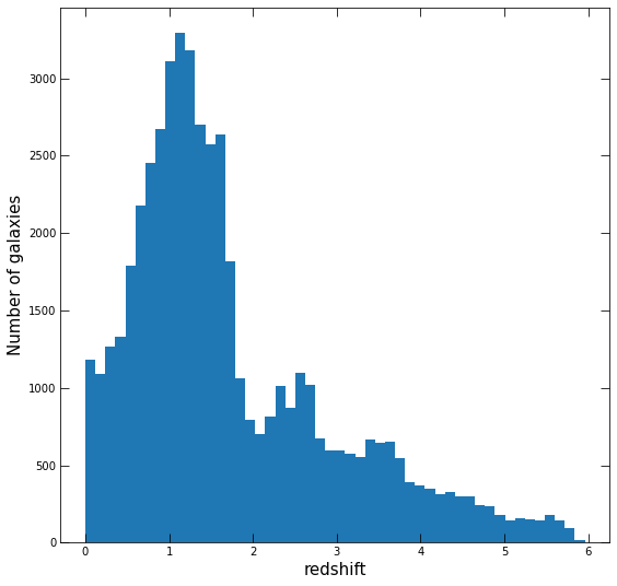
Let’s take a look at the redshift distribution of sources in the catalog.

There are several estimates of the photometric redshift, the one we want to use is z_peak for photometry, or, if available, z_spec_x, from spectroscopy.

What percentage of the catalog have measured spectroscopic redshifts? The z_spec_x column is set to -1 if no spectroscopic redshift exits.

(len(df.loc[df.z_spec_x!=-1,'z_spec_x']) / len(df))*100

2.86692933652761

Problem 2.5¶

Write a function get_redshift() which takes in an object ID, and returns z_spec_x for that source if it’s not -1, otherwise returns z_peak. Because id is a special word in python, we suggest using objid as the input, and setting df=df as an optional argument. You can make this a memory lite function by using df.loc[] to pull the row and only the two columns you need for this.

There are two additional “flagged” values: -99.0 and -99.9 – Have your function output np.nan if this is the value in the table.

Your function should return the redshift as well as a flag (string) ‘s’ or ‘p’, or ‘f’ for spectroscopic or photometric (or fail, if you’re returning nan).

def get_redshift(objid,df=df):
    options = df.loc[objid,['z_spec_x','z_peak']]
    if options.z_spec_x != -1:
        if options.z_spec_x != -99.0 and options.z_spec_x != -99.9:
            return options.z_spec_x, 's'
        else:
            return np.nan,'f'
    else:
        if options.z_peak != -99.0 and  options.z_peak != -99.9:
            return options.z_peak, 'p'
        else:
            return np.nan, 'f'

get_redshift(150)

(1.6689, 'p')

Problem 2.6¶

Now that we can get the best redshift for each row, use a list comprehension to grab these values for every object. You can index the output tuple of your function at 0 to drop the flag for now.

Once you have this, plot a histogram of the redshifts, using fig, ax = plt.subplots. Make your plot nice!

Note

My list comprehension takes ~15 seconds to run. It’s a lot of data! If you wish, you may try to find a more optimized solution built on a full column operation rather than a loop. One possibility is to take the spec-z column, mask any bad values, and then replace those entries in the z-phot column and plot that…

all_z = [get_redshift(i)[0] for i in df.index]

all_z = np.array(all_z)

fig, ax = plt.subplots(figsize=(9,9))
ax.hist(all_z[~np.isnan(all_z)],bins=50)
ax.set_xlabel('redshift',fontsize=15)
ax.set_ylabel('Number of galaxies',fontsize=15)
ax.tick_params(direction='in',top=True,right=True,length=8);

Problem 2.7¶

Now do the same, but separately plot the distributions of redshift for those with spectroscopic redshifts and those that only have photometric. For this, you’ll want to set density=True in your hist, and play with the linestyles and opacities so that both are visible.

Bonus (+0.5): Use KDE from seaborn to smoothly represent the distribution.

spec_z = [get_redshift(i)[0] for i in df.index if get_redshift(i)[1]=='s']; spec_z = np.array(spec_z)

phot_z = [get_redshift(i)[0] for i in df.index if get_redshift(i)[1]=='p']; phot_z = np.array(phot_z)

fig, ax = plt.subplots(figsize=(9,9))
ax.hist(spec_z,bins=40,density=True,alpha=0.9,label='Spectroscopic')
ax.hist(spec_z,bins=40,density=True,alpha=0.5,histtype='step',color='k',lw=3)

ax.hist(phot_z,bins=50,density=True,alpha=0.65,histtype='stepfilled',label='Photometric')
ax.hist(phot_z,bins=50,density=True,alpha=0.5,histtype='step',color='k',lw=3)

ax.set_xlabel('redshift',fontsize=15)
ax.set_ylabel('Number of galaxies',fontsize=15)
ax.legend(prop={'size': 16})
ax.tick_params(direction='in',top=True,right=True,length=8);

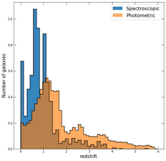
Do the differences between the two distributions make sense? Why or why not?

Note

Yes! We can see that the spectroscopic redshifts are clustered toward low redshift, while the tail of the photometric redshifts extends to higher redshift. This is because obtaining a spectrum is many times more observationally expensive than obtaining photometry, especially for many objects, and objects far enough away become too faint to measure in a survey of a set depth.

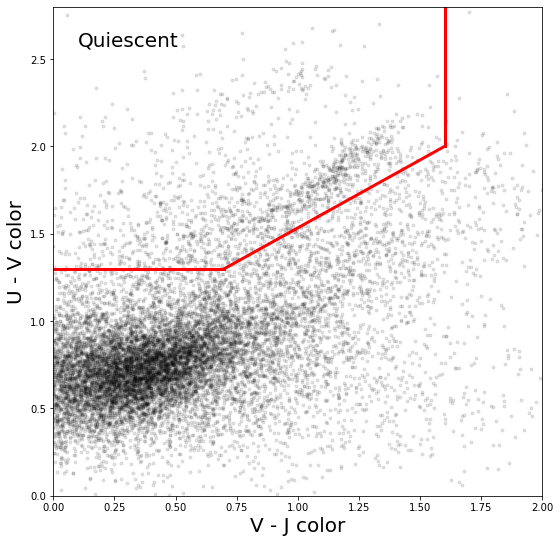
Problem 3¶

The “UVJ diagram” is a useful diagnostic tool in extragalactic astronomy which allows one to relatively accurately diagnose a galaxy as star forming or quiescent, even in the presence of dust. It is composed by plotting the “U-V” color of the galaxy against the “V-J” colors. You’ll likely know U and V (these are from the Johnsons-Cousin’s filter system). J is a filter in the near infrared.

In this problem, we’re going to write a function that can create a UVJ diagram for subsets of our data, cutting on mass and redshift.

You’ll need to access the following columns in the data (besides redshift, which you’ve already handled):

stellar mass: the mass of all the stars in the galaxy. (column: lmass, flagged value of -1)
star formation rate: rate at which galaxy is forming stars. (column: lsfr, flagged value of -99.0)
U band flux density (column: l153, flagged value of -99.0)
V band flux density (column: l155, flagged value of -99.0)
J band flux density (column: l161, flagged value of -99.0)

Problem 3.1¶

For step one, we need to be able to filter our dataframe for particular mass and redshift ranges.

Write a function, select_galaxies(), which takes as arguments M, delta_M, z, delta_z (and our dataframe). It should then return a df of only systems between M-deltaM to M+deltaM, and z-deltaz to z+deltaz. The columns it should return are the ones specified above.

There is actually a column in rf_df called z, that contains the spec_z if available or the peak z if not. At the time of writing, I cannot determine why this column was not included in the merge. In any case, set df['z'] equal to rf_df.z before continuing, as you’ll use it below.

Note

All masses and sfrs are in log units.

Try your function out using a mass of 10, delta M of 0.5 (i.e., a bin from 9.5 - 10.5), a redshift of 1, and a delta z of 0.25.

df['z'] = rf_df['z']

def select_galaxies(M,delta_M,z,delta_z,df=df):
    Mmin = M-delta_M
    Mmax = M+delta_M
    zmin = z-delta_z
    zmax = z+delta_z
    return df.loc[((df.lmass>Mmin)&(df.lmass<Mmax)&(df.z>zmin)&(df.z<zmax)),['lmass','lsfr','l153','l155','l161']]

select_galaxies(10,0.5,1,0.25)

	lmass	lsfr	l153	l155	l161
id
31	10.10	1.28	8.21804	19.45700	47.12630
56	10.00	1.32	5.85474	12.94060	29.94510
90	10.02	-1.15	4.85383	13.29640	32.60070
178	10.36	-1.90	1.94721	8.60585	49.25090
180	9.60	0.40	2.34370	4.87196	7.86611
...	...	...	...	...	...
50000	9.84	0.23	9.25872	21.86220	52.29720
50043	9.71	0.07	1.90277	5.09746	10.16970
50127	10.22	-0.08	17.21790	33.79470	70.21750
50180	9.96	-0.76	1.32408	6.03079	15.46360
50323	9.98	-2.84	1.74068	6.59796	14.86660

690 rows × 5 columns

Problem 3.2¶

Great, we can now get subsamples in mass/redshift bins. This is important because the UVJ diagram actually changes as a function of mass and redshift.

Next we need to get the colors out. Write a function get_colors() which takes the same arguments as your select_galaxies() function above. Inside, it should run select_galaxies passing through the arguments, and then from the resulting data frame, calculate U-V and U-J (see below). Add these as columns to said dataframe with names ‘U-V’ and ‘V-J’ and return it.

Run this function with the same mass/redshift bin from above and look at it.

Warning

As noted above, the U,V, and J band data are in Fnu (flux densities). Thus, a color is computed via -2.5*log10(Lfilter1/Lfilter2)

def get_colors(M,delta_M,z,delta_z,df=df):
    minidf = select_galaxies(M,delta_M,z,delta_z,df=df)
    minidf['U-V'] = -2.5*np.log10(minidf.l153/minidf.l155)
    minidf['V-J'] = -2.5*np.log10(minidf.l155/minidf.l161)
    return minidf

get_colors(10,0.5,0.75,0.25)

	lmass	lsfr	l153	l155	l161	U-V	V-J
id
31	10.10	1.28	8.21804	19.45700	47.12630	0.935769	0.960469
56	10.00	1.32	5.85474	12.94060	29.94510	0.861117	0.910928
90	10.02	-1.15	4.85383	13.29640	32.60070	1.094124	0.973732
178	10.36	-1.90	1.94721	8.60585	49.25090	1.613452	1.894051
180	9.60	0.40	2.34370	4.87196	7.86611	0.794504	0.520141
...	...	...	...	...	...	...	...
50000	9.84	0.23	9.25872	21.86220	52.29720	0.932857	0.946961
50043	9.71	0.07	1.90277	5.09746	10.16970	1.069919	0.749886
50127	10.22	-0.08	17.21790	33.79470	70.21750	0.732171	0.793992
50180	9.96	-0.76	1.32408	6.03079	15.46360	1.646150	1.022341
50323	9.98	-2.84	1.74068	6.59796	14.86660	1.446727	0.882005

690 rows × 7 columns

Problem 3.3¶

Now that we can easily grab U-V and V-J colors for subsamples, we’re ready to plot!

Next, set your xlim and ylim to (0,2) in V-J (x axis) and (0,2.8) in U-V (y axis).

Once you have the distribution plotted nicely, use the definitions of the bounding box provided in Whitaker et al. 2011 (Eqns 15, Fig 17 for example) to draw the box where quiescent galaxies sit.

fig, ax = plt.subplots(figsize=(9,9))
ax.set_box_aspect(1)
ob = get_colors(9.5,2,1.0,0.5)
ax.plot(ob['V-J'],ob['U-V'],'.',color='k',alpha=0.1);
ax.plot([0,0.7],[1.3,1.3],'r',lw=3)
ax.plot([1.6,1.6],[2.0,2.8],'r',lw=3)
ax.plot([0.7,1.6],[1.3,2.0],'r',lw=3)
ax.text(0.05,0.95,'Quiescent',ha='left',va='top',transform=ax.transAxes,fontsize=20)
ax.set_xlim(0,2)
ax.set_ylim(0,2.8)
ax.set_xlabel('V - J color',fontsize=20)
ax.set_ylabel('U - V color',fontsize=20)
ax.tick_params(direction )

Text(0, 0.5, 'U - V color')

Bonus (+2)¶

(+1) Now that you can easily plot up a UVJ diagram for a given mass/redshift bin, make a plot with 6 panels. Across the 3, plot the UVJ diagram in the redshift bins 0-0.5, 0.5-1.0, 1.0-2.0. In the top panel, include galaxies in the mass range 8-9.5, and in the bottom, 9.5-11.

(+1) Feeling extra fancy? Use the conditions on the UVJ quiescent box to color the quiescent galaxies red and the star forming galaxies blue in you plots.

Astro 330 Course Book

Lab 6: Solutions¶

Problem 1: HII regions + Planetary Nebulae measurements in M81¶

Problem 1.1¶

Problem 1.2¶

Problem 1.3¶

Problem 1.4¶

Problem 1.5¶

Problem 1.6¶

Bonus: (+1) Problem 1.7¶

Problem 2¶

Problem 2.1¶

Problem 2.2¶

Problem 2.3¶

Problem 2.4¶

Problem 2.5¶

Problem 2.6¶

Problem 2.7¶

Problem 3¶

Problem 3.1¶

Problem 3.2¶

Problem 3.3¶

Bonus (+2)¶