1. Astronomical Imaging & Functional Programming
Programming Topics: Functions, optional arguments, args and kwargs, documentation
Science Topics: filters/bands, multiband data, combinations, and continuum subtraction
Specialized Tools: Astropy tools for working with image data (SkyCoord, units, WCS, and Cutout2D)
Functional Programming
Everyone here is familiar with the idea of functions in Python. We import them (e.g., `np.array()`) and use them. We can also define our own functions. The standard function in python looks like
def func(args):
    '''
    Description of A function
    '''
    # Do something in the function
    return #something
Why write functional code? What concrete benefits arise from writing functions in our code?
My Answers
Prevents repetition of code that is run often
Allows for manual or automatic unit testing (ensuring each definable task in the code is working as expected)
Allows for double documentation. Functions themselves encourage docstrings, which helps users (you included) understand your function’s purpose. It also means your “main” code is composed fewer lines, due to calling functions instead. This makes the primary code easier to read, especially if the functions are well-named.
Functions are modular: you can import functions from one python file to another, the basic structure of package creation. (also works for classes)
Functions encourage simple outputs
Functions create regions of local scope, which helps prevent mucking up your global namespace
How to Write a Function
Besides the formatting, how do we actually construct good functions? How do we do so efficiently?
Playtest code in the global namespace (i.e., your script or notebook). When it’s working, move into a function.
Functions should be < 50 lines, and ideally < 20. They should handle simple, repetitive operations that don’t have many steps
A function wrapping several smaller functions is better than one long function
Anytime you find yourself copying and pasting code, you could probably use a function
Don’t write detailed docstrings until the function is “mature”. #Comments throughout are sufficient.
Because you won’t have to type them out often, variable names in functions can be highly descriptive.
It’s better to let the code guide when to make functions, rather than forcing all code into functions a priori.
Documentation
Documentation is one of the most important things we create as programmers. It is the number 1 descriminator in whether a codebase remains useful over any extended period of time.
I consider all of the following documentation
variable names
function and class names
#inline comments
docstrings for classes, methods, and functions
Docstrings are the most formal form of documentation. These are descriptions of scripts, methods, classes, and functions which are typically written in one of several standard methods.
The docstring styling is important, because there are automated programs such as Sphinx and mkdocs which can analyze your code base and construct documentation websites for you.
We’ll be using the numpy/scipy in this class. It is a standard styling which is compatible with the tools listed above and is easy to write and read. It looks like this:
def func(arg1,arg2,arg3=0,**kwargs):
    '''
    A function which does something with three optional arguments and some keyword arguments

    Parameters
    ----------
    arg1: float
        description of arg1, which has been indicated to be a float
    arg2: array_like
        description of arg2, which has been indicated to be an array
    arg3: int, optional
        description of arg3, an optional input. Default: 0
    **kwargs: dict_like, optional
        Any additional keyword arguments will be stored in the functions kwargs dictionary.

    Returns
    -------
    output1, output2: int, float
        This function returns 2 outputs, one an int and one a float, apparently.

    Notes
    -----
    Requires numpy version >1.15.5
    Notes go here

    See Also
    --------
    Any links to other functions can go here
    '''
    pass
I definitely don’t write that level of documentation for most of my functions (at least not as I’m writing them). My docs, when I’m playtesting code, usually look more like
def func(a,b,c):
    # Does Calculation X using a,b,c, which should be floats
    pass
Then, once the function has been fleshed out, and I know for (mostly) sure that the inputs and outputs I want are stable, I’ll write up the more official docstring from above. In writing code for myself or colleagues (i.e., not distributed), notes and see also is generally overkill. But the basic docs laying out parameters and returns is worth doing. Here’s a website built using automatic docstrings.
*Args and **kwargs
The simplest version of a Python function includes several ordered inputs, defined in the def line of the function definition. One step higher in complexity, after the ordered arguments, one can add optional or keyword arguments, which have set defaults but can be overwritten by the user by entering an argument with the appropriate keyword, via kw=something.
These methods are likely familiar. Less familiar may be the use of *args and **kwargs as inputs to your functions.
In the simplest sense, these arguments are packing and unpacking variables. As a reminder about unpacking and packing, let’s look at an example:
theta = (1,5,3,6,7,3)
def func(theta):
    a,b,c,d,e,f = theta
In the code above, we “packed” theta into an iterable containing subparts, and read this container into func. We then unpacked it by setting 6 variables all equal to theta. This works only if the number of variables equals the length of the input.
Tuples are the default for packing things, but any simple iterable (like a list) work. Here’s another example:
def func():
    a = 2
    b = 5
    return a,b
By returning a,b, we are actually telling python to pack the outputs into a tuple. If we then run out function by setting a single variable, via out = func(), then out will be a tuple containing two items. But we can also run our function via c,d = func(), and it will unpack that tuple directly into the two variables specified.
As a random side note, one of our favorite functions, np.where(), returns a tuple containing the indices of interest and then, usually, nothing. Hence, you’ll often see people run where as
w, = np.where(somthing>something_else)
That comma tells python to unpack the tuple, and the lack of a second variable tells it to simply dump whatever the second output is.
Packing and unpacking are key to our use of args and kwargs in functions. But first, why use them at all?
You may want to allow any number of inputs to your function
You may want to pass arguments from your function to another.
Matplotlib is a classic example of a library with many **kwarg enabled functions. When we use wrappers that conveniently allow a complex plot to be made in one line, we still want to be able to put in parameters that alter or set more granular settings.
By adding **kwargs as an optional input to our functions, the user can supply any number of extra keyword/arg pairs. These sit harmlessly in a dictionary called kwargs. If then inside our function we call another function which has **kwargs enabled, we can then feed our kwargs dict into that function, and unpack it into keyword argument pairs again with the **.
Example
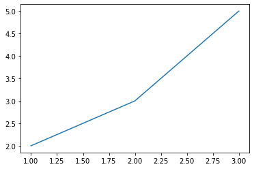
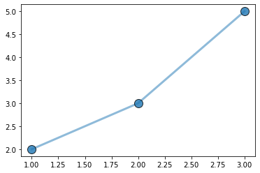
import matplotlib.pyplot as plt
def plot_wrapper(x,y,**kwargs):
    fig, ax = plt.subplots()
    ax.plot(x,y,color='C0',**kwargs)
x = [1,2,3]
y = [2,3,5]
plot_wrapper(x,y)
x = [1,2,3]
y = [2,3,5]
plot_wrapper(x,y,lw=5,alpha=0.5)
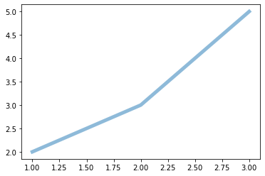
Notice that when I run plot_wrapper, I’m passing in arguments accepted by ax.plot, and since I feed **kwargs into ax.plot inside my function, it passes through to the plot command.
Checking kwargs
In the above example, we blindly fed all kwargs of plot_wrapper into ax.plot. So If I were to add a kwarg to plot_wrapper that is not a kwarg of ax.plot(), I’d get an error.
We can be more careful by either demanding a dictionary input for matplotlib commands specifically, or we can check the keys of kwargs manually and ensure that we only pass the relevant ones along.
Since we can’t be sure which of the many inputs a user would use, in this case, it makes most sense to demand a dict. We still use the magic of unpacking to take that dictionary and pass it into the plotting command as key-value pairs, though.
def plot_wrapper(x,y,line_args={},symb_args={}):
    fig, ax = plt.subplots()
    ax.plot(x,y,color='C0',**line_args)
    ax.plot(x,y,'o',color='C0',**symb_args)
plot_wrapper(x,y)
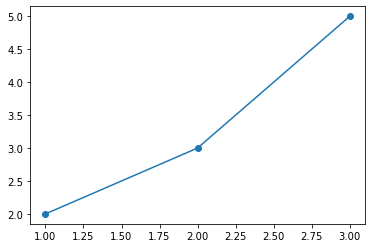
plot_wrapper(x,y,line_args={'lw':3,'alpha':0.5},
                 symb_args={'ms':12,'mec':'k','alpha':0.8})
Notice that normally, one can’t feed a dictionary of key-values into a function. ax.plot() expects the keywords to look like (...,lw=3,alpha=0.5). But because we used ** on our dict, we unpacked it into the function.
So, to summarize: ** packs up a key=value pairs when used in a function definition, storing in a dict called kwargs, and then using **kwargs again in the call (rather than definition) of another function will unpack that dictionary and pass the inputs to the function as desired.
Working with Images
Now that we’re caught up on our function definitions, documentation, and fancy use, let’s dive into the science part: images!
What’s in an image
Astronomical images differ from standard images taken with a phone or DSLR camera primarily in that they both use older CCD technology and are typically “black and white”, recording only intensity of light and not color.
Knowledge about color instead comes from the placement of filters in front of the detectors which have a certain bandpass, allowing through light within a certain wavelength range and blocking light outside it.
Thus, we only ever get one color at a time, unless the telescope splits incoming light by color using, for example, a dichroic, and then sends the two streams to two detectors with different filters simultaneously.
This means that in some sense, single-band (i.e., one narrow-ish wavelength range) images are simple programmatically: They are 2D arrays in which each pixel (position in array) contains a single number: counts (in some units).
Usually, these units are counts in ADU (analog-to-digital units), which are roughly related to the actual counts of photons hitting the detector, via properties such as the gain of the system.
Generally, we are not concerned with the exact units/gain/etc., because we back out the flux in photons (or energy, rather) via empirical calibrations with objects in the sky of known flux.
Narrowband Data and Continuum Subtraction
Many astronomical surveys are carried out with broadband filters, such as U,B,V,R,I or Sloan-u,g,r,i,z. These wide filters let in a lot of light, making for quicker observations.
Narrowband filters, meanwhile, are generally used to target emission lines from gas. This includes the famous \(H\alpha\) line, along with other ionization lines.
Narrowband filters attempt to block all light except that just surrounding the emission line. But the emission seen (at some wavelength targeting a line) is the superposition of the emission line and the stellar continuum (i.e., the star light also coming from the galaxy/region).
Thus, to use narrowband data properly, it must be continuum subtracted. Generally, this is done by scaling a broadband image also encompassing the line (so for \(\lambda\)6563 \(H\alpha\). \(R\)-band) and then subtracting it from the narrowband image.
Breakout Question: Discuss with your partner an obvious problem with recovering emission line fluxes using this method.
Why bring this up?
In Lab 2, we’ll be working with a set of HST images in different bands, including \(H\alpha\), and you’ll have to perform a continuum subtraction.
When working directly with images, the primary mode of operation is the measurement of flux in different regions on the sky – in both broadband, and narrowband data.
Image Handling with Astropy
Lastly, we need to know how to work with astronomical images in Python. As “simple” 2D arrays, simply opening and plotting an image is easy. But keeping track of, say, the celestial coordinates associated with a pointing on the sky, is not.
Luckily, the open-source astropy library has many tools that facilitate the streamlined handling of astronomical imaging.
Opening the Image
Opening images using astropy is made easy using the fits file handler. We’ll use a context manager to read in an image:
from astropy.io import fits

with fits.open('antenna_Rband.fits') as hdu:
    header = hdu[0].header
    image = hdu[0].data
We can confirm we’ve loaded a 2D array:
image
array([[ 4.8691406,  5.432617 ,  5.713867 , ..., 11.48584  , 11.48584  ,
        11.48584  ],
       [ 5.573242 ,  5.713867 ,  5.291504 , ..., 11.48584  , 11.48584  ,
        11.48584  ],
       [ 6.4179688,  5.573242 ,  5.573242 , ..., 11.48584  , 11.48584  ,
        11.48584  ],
       ...,
       [11.48584  , 11.48584  , 11.48584  , ...,  6.2768555,  5.432617 ,
         5.9956055],
       [11.48584  , 11.48584  , 11.48584  , ...,  5.291504 ,  5.432617 ,
         5.573242 ],
       [11.48584  , 11.48584  , 11.48584  , ...,  5.291504 ,  4.8691406,
         3.4614258]], dtype=float32)
We can make a basic plot showing it:
fig, ax = plt.subplots(figsize=(6,6))
ax.imshow(image)
<matplotlib.image.AxesImage at 0x7fcfd9379bb0>
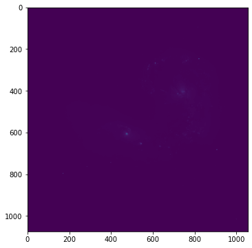
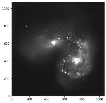
That may not have looked like much, but it did at least confirm we have a 2D image. Let’s tweak some settings.
import numpy as np
fig, ax = plt.subplots(figsize=(6,6))
m = np.mean(image)
s = np.std(image)
ax.imshow(image,origin='lower',vmin=m-s,vmax=m+5*s,cmap='gray');
Next, we need to plot with our \(x\) and \(y\) axes representing sky coordinate (RA/DEC) rather than pixel position. For this, we’ll need to use astropy’s World Coordinate System module. There are several defined coordinate systems on the sky, but for this class, we’ll primarily be using RA and DEC. (i.e., equitorial coordinates measured in hour angles and degrees).
from astropy.wcs import WCS

wcs_im = WCS(header)
INFO:
                Inconsistent SIP distortion information is present in the FITS header and the WCS object:
                SIP coefficients were detected, but CTYPE is missing a "-SIP" suffix.
                astropy.wcs is using the SIP distortion coefficients,
                therefore the coordinates calculated here might be incorrect.

                If you do not want to apply the SIP distortion coefficients,
                please remove the SIP coefficients from the FITS header or the
                WCS object.  As an example, if the image is already distortion-corrected
                (e.g., drizzled) then distortion components should not apply and the SIP
                coefficients should be removed.

                While the SIP distortion coefficients are being applied here, if that was indeed the intent,
                for consistency please append "-SIP" to the CTYPE in the FITS header or the WCS object.

                 [astropy.wcs.wcs]
WARNING: FITSFixedWarning: 'datfix' made the change 'Set MJD-OBS to 53207.000000 from DATE-OBS'. [astropy.wcs.wcs]
The wcs for a given image is constructed from the image header, where some information about the pixel scale and image pointing are stored. Notice here we got a warning. This happens sometimes with HST images that are mosaics of pointings that have already been drizzled (an image alignment/combination process). We need to remove the mentioned coefficients.
The following will be provided for lab:
def strip_SIP(header):
    A_prefixes = [i for i in header.keys() if i.startswith('A_')]
    B_prefixes = [i for i in header.keys() if i.startswith('B_')]
    for a,b in zip(A_prefixes,B_prefixes):
        del header[a]
        del header[b]
    return header
header_fixed = strip_SIP(header)
wcs = WCS(header_fixed)
We are now ready to plot our image in celestial coordinates. Our game plan is to use matplotlib’s projection. You may be familiar with this as the way to make an axis, e.g., in polar coordinates. Astropy WCS objects can be treated as projections in matplotlib. Below I show two ways to initialize an axis with our new wcs projection.
fig, ax = plt.subplots(figsize=(6,6),subplot_kw={'projection':wcs})
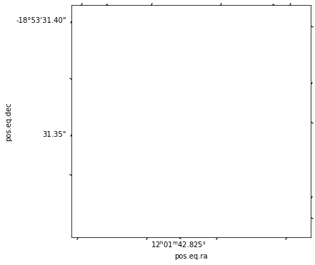
fig = plt.figure(figsize=(6,6))
ax = fig.add_subplot(projection=wcs)

The two methods work equally well. The former is slightly preferred, as it makes it easy to make multiple panels with a wcs projection.
Now, all we have to do, is plop our image into it:
fig, ax = plt.subplots(figsize=(6,6),subplot_kw={'projection':wcs})
ax.imshow(image,origin='lower',vmin=m-s,vmax=m+5*s,cmap='gray');
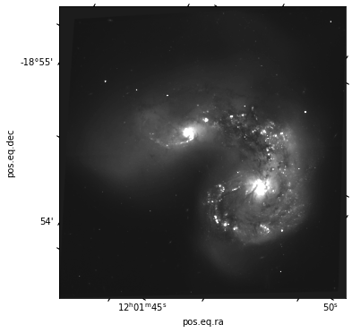
ax
<WCSAxesSubplot:xlabel='pos.eq.ra', ylabel='pos.eq.dec'>
Lab Preview
In the lab, you’ll be working with the same image of the Antenna galaxy, in several bands. In addition to the basic reading in and use of header/wcs, you’ll be learning about SkyCoord, the astropy handler for coordinates, and units which is a module we’ll be discussing throughout class. You’ll use Cutout2D to make zoom in plots of the image while retaining coordinate information. And you’ll use the photutils package and sep to find sources and perform some aperture photometry.